Ask for the relevant numbers, their meanings and units, and the decision to support, then choose the matching equation. For profile questions, compare size and direction separately. For table simplification, report compression error alongside retained squared norm. For forecasts, check probability support before scoring. For sensitivity questions, show a local derivative and a finite-change check. For sample-size questions, state the range of the data and whether a worst-case or typical-case guarantee is wanted. Return only the relevant calculation in a form the reader can reproduce.
“My weekly activity profiles are (3, 4) and (6, 8) hours for the same two activities. Did my workload change, my balance of activities change, or both?”
Use mathllms-ch01-foundations with the companion's AI skill package. The illustrations below also work on their own.
Which part of a profile should count as size?
From Chapter 1, The Shape of Measuring
If a profile doubles but keeps its proportions, which comparisons should change?
A norm answers how large a vector is under a chosen rule: total absolute activity, straight-line size, or the largest component. The unit ball shows all profiles of size exactly one under that rule, and dividing x by its size lands it on the ball. Cosine divides away length, so it identifies similar proportions even when amounts differ greatly.
Predict first: Before setting scale to 2, predict whether the selected size, the distance to y, the dot product and the cosine will each double.
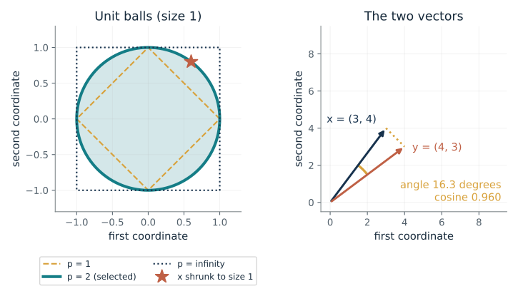
Measuring rule (p): 2 · Scale of (3, 4): 1
What happens: The size doubles (5 to 10) and the dot product doubles (24 to 48), but the cosine stays at 0.96 and the angle at 16.3 degrees. The distance to y does not double: it goes from 1.41 to 5.39, because y did not move.
With p = 2, x has size 5 and sits 1.41 from y. Changing the scale changes sizes and the dot product, but the angle between x and y stays at 16.3 degrees.
- Size of x (p = 2)
- 5
- Distance from x to y (p = 2)
- 1.41
- Dot product of x and y
- 24
- Cosine of the angle
- 0.96
Embedding similarity in language models is usually a cosine because direction carries the meaning while vector length mostly reflects frequency and training details. Choosing the wrong measuring rule changes which items count as close.
Show the calculation
Size of x = sqrt(3^2 + 4^2) = 5. Dot product = 3 x 4 + 4 x 3 = 24. Lengths: |x|_2 = 5, |y|_2 = 5. Cosine = 24 / (5 x 5) = 0.96. Distance = |x - y| with x - y = (-1, 1), measured with the same p.
The equations and symbols
- x
- the profile being measured, scale times (3, 4)
- y
- the comparison profile, fixed at (4, 3)
- p
- measuring rule: 1 adds, 2 is straight-line, infinity takes the largest
- d_p
- distance between x and y under rule p
- theta
- angle between x and y; cosine has no units
Finite real coordinates and p >= 1. Cosine requires both vectors to be nonzero; the scale-zero state displays it as undefined. Positive scaling preserves angle. The axes share units; a norm is not automatically meaningful for mixed units. Infinity means the largest coordinate, not a large finite p.
Check your understanding: For x = (3, 4), what are the three norms, and can a cosine of 1 tell you whether the recorded hours are accurate?
Book source: Chapter 1, The Shape of Measuring. Illustration C01-D01. Identity. Book definitions; (3, 4), (4, 3), and the scale controls are illustrative hand calculations. v39 EPUB / v43 print.
How much error does one discarded direction cost?
From Chapter 1, The Skeleton of Every Matrix; The Best Possible Compression
How closely can a rank-k table reproduce the book's three-by-three matrix?
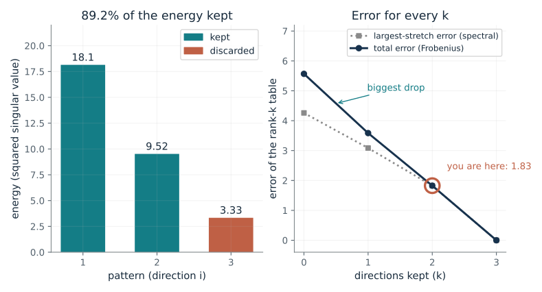
SVD writes the table as a sum of ranked patterns, each with a strength. Keeping the strongest k patterns gives the smallest possible error among all tables of that rank. The error is the square root of the energy in the patterns you drop, and the bar chart shows exactly which energy that is.
Predict first: Which direction holds more energy, the first or the third, and does the total error fall by more when you add the first or the third?
Patterns kept (k): 2 · Error measure: total
What happens: The first direction holds far more energy: 18.1 of the 31 units against 3.33 for the third, so keeping only it already holds 58.5% of the energy and drops the total error from 5.57 to 3.59 (a drop of 1.98, against 1.83 for the third). Energy shrinks steadily from direction to direction, but the error drops stay nearly equal, so the error curve is close to a straight line.
Keeping 2 of 3 directions keeps 89.2% of the energy; only the weakest pattern is dropped, so the total error 1.83 equals the largest-stretch error and the two curves meet.
- Energy kept
- 89.2%
- Total error (Frobenius)
- 1.83
- Largest-stretch error (spectral)
- 1.83
- Singular values
- 4.26, 3.09, 1.83
Low-rank adapters (LoRA) and compressed embedding tables rely on this: keep the top few singular directions and the rest of the weight matrix costs little. The leftover energy tells you what the compression gives up.
Show the calculation
Energy: 4^2 + 1^2 + 3^2 + 1^2 + 2^2 = 31 = 18.1 + 9.52 + 3.33. Kept 27.7 of 31 = 89.2%. Total error = sqrt(3.33) = 1.83. Largest-stretch error = singular value k+1 = 1.83. Rank-2 table rows: (3.98, 1.06, -0.11); (0.09, 2.72, 1.50); (-0.26, 0.83, 0.51).
The equations and symbols
- A
- the book matrix [[4,1,0],[0,3,1],[0,0,2]]
- sigma_i
- singular value i: how strongly pattern i appears, largest first
- k
- number of patterns kept
- A_k
- the best table built from the top k patterns
- energy
- squared singular value; the total is 31
Finite real matrix and integer 0 <= k <= rank(A). The guarantee applies to approximation rank at most k under the stated norms. Retained energy is a squared Frobenius-norm fraction; it does not measure semantic importance or file compression. Numerical reconstruction can leave machine roundoff at full rank, shown here as 0.
Check your understanding: If k = 0, what is the approximation and its total error? What happens at k = 3?
Book source: Chapter 1, The Skeleton of Every Matrix; The Best Possible Compression. Illustration C01-D02. Theorem. Book matrix and Eckart-Young error identity. Singular values are recomputed at full numerical precision rather than copied from rounded prose. v39 EPUB / v43 print.
How much does a mistaken forecast add to surprise?
From Chapter 1, The Price of Being Wrong About a Distribution
Which part of a forecast's average log loss comes from uncertainty, and which part comes from mismatch?
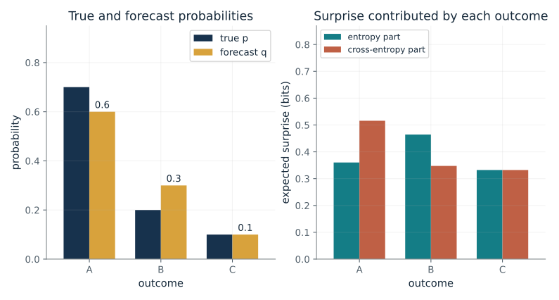
Entropy is the average surprise inherent in the population. Cross-entropy evaluates outcomes from that population using the forecast's probabilities, so a poor forecast adds a penalty. The identity splits that total exactly; changing the logarithm base changes the units while preserving the split.
Predict first: If q is changed to match p, does average surprise disappear, or does only the mismatch penalty disappear?
Forecast q: book · Logarithm units: bits
What happens: Only the penalty disappears. The forecast bars equal the true bars, KL is 0, but cross-entropy still equals the entropy, 1.16 bits, because outcome C still happens by chance.
Total surprise 1.2 bits splits into entropy 1.16 plus a mismatch penalty of 0.0387. A perfect forecast removes only the penalty; the entropy stays because the world itself is uncertain.
- Entropy H(p), the unavoidable part
- 1.16 bits
- Mismatch penalty (KL)
- 0.0387 bits
- Cross-entropy, the total
- 1.2 bits
- Forecast q
- 0.6, 0.3, 0.1
A language model is trained by minimizing cross-entropy on text. The floor of that loss is the entropy of the text itself, so a loss that stops falling may mean the model matches the data, not that training failed.
Show the calculation
Outcome A: -0.7 x log2(0.6) = 0.516. Adding all three terms gives cross-entropy 1.2. Entropy = 1.16. Penalty = 1.2 - 1.16 = 0.0387.
The equations and symbols
- p
- true outcome probabilities, fixed at (0.7, 0.2, 0.1)
- q
- the forecast probabilities for outcomes A, B, C
- H(p)
- entropy: average surprise nobody can avoid
- H(p,q)
- cross-entropy: average surprise using the forecast
- D_KL
- extra surprise caused by the forecast being wrong
- b
- log base: 2 gives bits, e gives nats
Both distributions are nonnegative and normalized on the same finite outcomes. Terms with p_i = 0 contribute zero. If p_i > 0 and q_i = 0, cross-entropy and KL are infinite. Finite KL is nonnegative for the log bases used here and is generally asymmetric.
Check your understanding: Why can one outcome contribute a negative term to KL while total KL stays nonnegative?
Book source: Chapter 1, The Price of Being Wrong About a Distribution. Illustration C01-D03. Identity. Book distribution pair p = (0.7, 0.2, 0.1), q = (0.6, 0.3, 0.1); matched and zero-probability forecasts are illustrative boundary cases. v39 EPUB / v43 print.
Trace a change through two stages
From Chapter 1, The Algorithm That Learns by Looking Backward
How does a small change in the input pass through a composed function?
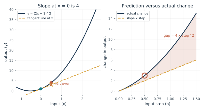
The first stage multiplies a small input change by 2. The second multiplies the resulting middle change by its local slope 2u, so the composed slope is their product. Backpropagation repeats this accounting across many operations; it does not make a curved function globally linear.
Predict first: At x = -0.5, the slope is zero. Predict whether a positive finite step leaves y exactly unchanged.
Starting input (x): 0 · Input step (h): 0.5
What happens: No. The slope-based prediction is 0, yet the output rises by 4 (from 0 to 4). The whole change is the left-over curvature term 4h squared, which is why the right panel shows a curve while the prediction stays flat.
At x = 0 the slope is 4, predicting a change of 2. The actual change is 3; the gap 1 is curvature, and it grows with the square of the step.
- Chain-rule slope (2u) x 2
- 4
- Predicted change (slope x step)
- 2
- Actual change
- 3
- Left over (curvature)
- 1
Backpropagation is this chain-rule bookkeeping repeated through every layer of a network. A gradient step is a small step along that slope, so a learning rate that is too large lands in the curvature gap.
Show the calculation
u = 2(0) + 1 = 1. Slope = (2u) x 2 = 2 x 2 = 4. Predicted change = 4 x 0.5 = 2. Actual: y goes from 1 to 4, a change of 3. Left over = 4 x 0.5^2 = 1. Matrix version: with f(X) = (2X1 + X2, X1 - X2) and g(u) = (u1^2 + u2, u1 u2) at X = (0, 1), Jg(f(X)) times Jf(X) has rows (5, 1); (-1, -2).
The equations and symbols
- x
- the input
- u
- the middle value after stage one, 2x + 1
- y
- the output, u squared
- h
- the size of the input step
- J
- Jacobian: table of slopes, rows are outputs, columns are inputs
Both stages are differentiable everywhere. The derivative product is exact; derivative times a finite step is a local approximation. The exact remainder here is 4h squared. A zero derivative at the minimum does not mean every finite step leaves the output unchanged. All quantities are dimensionless.
Check your understanding: At x = 0 and h = 0.5, what are the predicted and actual output changes?
Book source: Chapter 1, The Algorithm That Learns by Looking Backward. Illustration C01-D04. Identity. Book chain-rule, Jacobian, and local-linearization principles; the scalar u = 2x + 1 followed by u squared and the displayed two-dimensional f and g are illustrative compositions. v39 EPUB / v43 print.
How many samples make a 95% guarantee?
From Chapter 1, The Tools for Measuring Concentration (Worked example: Sample size for 95% confidence)
If I average n answers that each lie between 0 and 1, how often can the average miss the truth by 0.05, and how many answers do I need to be sure?
An average of many independent bounded answers rarely strays far from the truth. Hoeffding turns that into a ceiling on the miss chance that falls exponentially with n. Because it must hold for every possible source, it cannot use the actual variance, so it is looser than a calculation that does.
Predict first: The bound says 738 samples guarantee a miss chance of at most 5%. Predict whether the simulated miss rate at n = 738 will be near 5%, above it, or far below it.
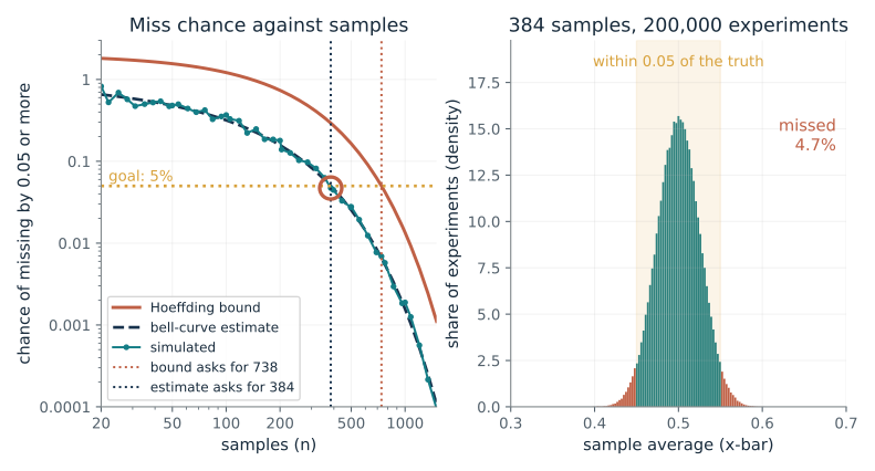
Samples (n): 384 · Chance an answer is 1 (q): 0.5
What happens: Far below: about 0.7%, while the bound sits exactly at 5%. The bell-curve estimate needs only 384 samples to reach 5%. The bound is safe for any bounded source, and that safety costs about twice as many samples.
At n = 384 the bound allows a miss chance up to 0.293, while the simulation misses 0.0471 of the time. The bound is safe but loose, because it must hold for every source between 0 and 1. The bell-curve estimate is 1.06 times the simulated value; the bound is 6.22 times it.
- Hoeffding bound on the miss chance
- 0.293
- Simulated miss chance
- 0.0471
- Bell-curve estimate
- 0.05
- Samples the bound asks for
- 738
Evaluating a language model on a test set of n questions is exactly this average. The bound says how many questions guarantee that a measured accuracy is within 5 points, and the gap to the simulation shows how much that guarantee costs.
Show the calculation
Bound = 2 exp(-2 x 384 x 0.05^2) = 2 exp(-1.92) = 0.293. Samples for a 5% bound: n = ln(2 / 0.05) / (2 x 0.05^2) = ln(40) / 0.005 = 3.69 / 0.005 = 738, so 738. Bell-curve estimate: spread of the average = sqrt(0.5 x 0.5 / 384) = 0.0255; miss chance = 2 x P(Z > 0.05 / spread) = 0.05. Samples by the bell curve: 1.96^2 x 0.25 / 0.05^2 = 384.
The equations and symbols
- n
- number of independent answers averaged
- epsilon
- allowed miss, fixed at 0.05
- delta
- allowed chance of missing by more than epsilon, fixed at 0.05
- q
- chance a coin-flip answer is 1; sets how much the answers vary
Independent answers in [0, 1]. Hoeffding needs no knowledge of the variance, which is why it is conservative. The bell-curve estimate uses the true variance q(1 - q) and is an approximation, not a guarantee. Simulated rates carry roughly 0.1% noise at the 5% level and are noisier for very small rates.
Check your understanding: For accuracy epsilon = 0.1 instead of 0.05 and the same delta, how many samples does Hoeffding ask for?
Book source: Chapter 1, The Tools for Measuring Concentration (Worked example: Sample size for 95% confidence). Illustration C01-D05. Theorem. Book worked example (epsilon = delta = 0.05, 738 and 384 samples). The simulation uses 200,000 seeded repeats of n coin flips with chance q; q values are illustrative. v39 EPUB / v43 print.
How few dimensions can keep every distance?
From Chapter 1, When High Dimensions Surprise
If 40 points live in 500 dimensions, how many random directions do I need to keep all their pairwise distances nearly right?
A random direction sees each distance as a sum of many small independent contributions, so its squared length concentrates around the true value. Averaging k such directions narrows the spread like the square root of 2/k. With only 40 points there are 780 pairs, and a union bound over them costs only a logarithm.
Predict first: Starting from 500 dimensions, how many dimensions k do you expect to need before every pair of the 40 points stays within 50% of its true squared distance?
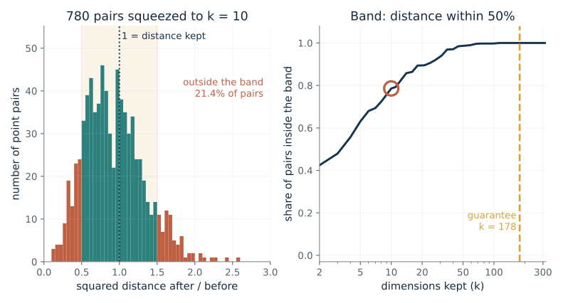
Dimensions kept (k): 10 · Allowed distortion (epsilon): 0.5
What happens: At k = 160 every pair is inside the band, so about a third of the original dimension suffices; the theorem's guarantee is 178. At k = 10 about a fifth of the pairs fall outside, and at k = 2 more than half do.
At k = 10 only 79% of the pairs stay within 50%. The ratios scatter around 1 with spread about 0.447; more dimensions narrow the scatter, and the theorem guarantees all pairs at k = 178.
- Pairs inside the band
- 78.6%
- Smallest ratio seen
- 0.143
- Largest ratio seen
- 2.58
- Dimensions the theorem guarantees
- 178
Embedding tables and attention keys are compared millions of times; random projection (and hashing tricks built on it) shrinks them while keeping similarity scores nearly intact. The cost is a controlled, quantifiable error.
Show the calculation
Each pair's ratio has average 1 and spread sqrt(2/k) = sqrt(2/10) = 0.447. Band: [0.5, 1.5]. Guarantee: k >= 4 ln(40) / (0.5^2/2 - 0.5^3/3) = 14.8 / 0.0833 = 178. Seeded run: 40 random points in 500 dimensions, one Gaussian projection with entries of variance 1/k.
The equations and symbols
- x_i
- one of 40 points in 500 dimensions
- A
- random k-by-500 map with Gaussian entries of variance 1/k
- k
- dimensions kept after the map
- epsilon
- allowed relative distortion of squared distances
- ratio
- squared distance after the map divided by before
Fixed finite point set, Gaussian random map, epsilon in (0, 1/2] for the guarantee formula (the 0.5 state is its boundary). The guarantee holds with high probability over the draw of A, not for every A. Distances between the 40 listed points only; new points are not covered.
Check your understanding: If you double the number of points to 80, roughly how does the guaranteed k change?
Book source: Chapter 1, When High Dimensions Surprise. Illustration C01-D06. Theorem. Book Johnson-Lindenstrauss theorem. The guarantee formula is the Dasgupta-Gupta form of the same bound. Points, projection, and seed 7 are an illustrative simulation. v39 EPUB / v43 print.
When does an average of skewed draws look like a bell?
From Chapter 1, The Geometry of Probability Families (Theorem 1.3, Central Limit Theorem)
The source is lopsided. How many draws must I average before the result is close to a bell curve?
One draw from a lopsided source has a long tail on one side. Averaging n draws shrinks the spread by the square root of n and the lopsidedness by the same factor, so the standardized average slowly approaches the symmetric bell. The right panel measures the leftover distance exactly, for both sources.
Predict first: For an exponential source (skewness 2), how many draws must you average before the largest gap to the bell curve falls below 0.03?
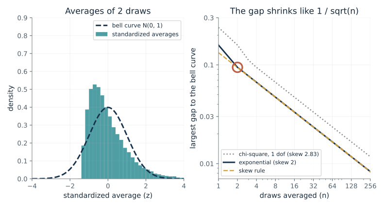
Draws averaged (n): 2 · Source: exponential
What happens: About 32 draws: the gap is 0.024 at n = 32 and 0.033 at n = 16. The histogram now hugs the bell curve. The chi-square source, with higher skew, is still at 0.033 there.
With only 2 draws the average keeps the lopsided shape of the source: the bell curve is off by up to 0.0945 in probability. Skewness fades only as 1 divided by the square root of n.
- Skewness of the average
- 1.41
- Largest gap to the bell curve (exact)
- 0.0945
- Chance of landing above +2 (simulated)
- 4.9%
- Same chance for a bell curve
- 2.28%
Error bars on benchmark scores, on gradient noise in minibatches, and on loss averages all assume this bell shape. For heavy, lopsided errors the shape is not yet a bell at small batch sizes, so intervals can be wrong.
Show the calculation
Source skewness = 2. Average of 2: skewness = 2 / sqrt(2) = 1.41. Skew rule for the gap = skew / (6 sqrt(2 pi n)) = 2 / (6 x 3.54) = 0.094; exact gap = 0.0945. Standardized average: z = (average - mean) / (spread / sqrt(n)), simulated with 20,000 seeded repeats.
The equations and symbols
- n
- number of draws averaged
- mu, sigma
- mean and spread of one draw
- Z_n
- the average, centred and divided by its spread (standardized)
- gamma
- skewness of one draw: 2 for exponential, 2.83 for chi-square with 1 dof
- Phi
- the standard bell-curve cumulative probability
Independent identical draws with finite variance. The theorem is a limit; at finite n the error depends on the source's skewness, and the first-order rule is accurate only for moderate to large n. The simulated histogram shows sampling noise of a few percent per bin.
Check your understanding: A source has skewness 4, twice the exponential. About how many draws does it need to reach the same gap as the exponential at n = 32?
Book source: Chapter 1, The Geometry of Probability Families (Theorem 1.3, Central Limit Theorem). Illustration C01-D07. Theorem. Book central limit theorem. Sources are exponential and chi-square (gamma family); histograms use 20,000 seeded repeats, while the gap is computed exactly from the gamma distribution. The skew rule is the first Edgeworth correction. v39 EPUB / v43 print.
How little can an estimate wobble?
From Chapter 1, The Geometry of Probability Families (Worked example: Fisher information for logistic regression; Theorem 1.4)
When I fit a logistic regression to n examples, how widely do the fitted weights scatter, and is there a floor below which no unbiased method can go?
Fisher information measures how sharply the likelihood peaks around the true weight. A sharper peak means less wobble from sample to sample, and the wobble cannot go below 1 over n times the information. A larger true weight pushes more predictions toward 0 or 1, where one example barely moves the likelihood, so the floor rises.
Predict first: After you increase n from 50 to 1,600, will the scatter of the fitted weights fall to match the 1 / (nF) floor, or stay well above it?
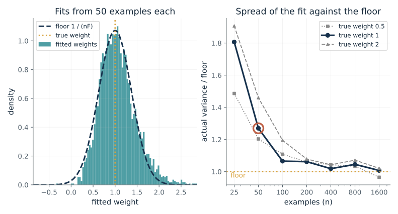
Examples per fit (n): 50 · True weight (w): 1
What happens: It matches: the actual variance is within a few percent of the floor, and the histogram sits under the dashed floor curve. At n = 50 it was about 1.3 times the floor, so small samples are noisier than the floor suggests.
With 50 examples the fitted weights scatter about 1.27 times the floor variance: the floor is a limit for large samples, and small samples are well above it. More examples bring the ratio toward 1.
- Information per example F
- 0.144
- Floor 1 / (n F)
- 0.139
- Actual variance of the fits
- 0.176
- Actual / floor
- 1.27
Fisher information is the curvature that natural-gradient and second-order optimizers use. A saturated neuron has low information, which is the same fact as vanishing gradients: examples there tell the model almost nothing new.
Show the calculation
For x ~ N(0, 1), F(w) = E[s(1 - s) x^2] with s = 1 / (1 + e^(-w x)); numerical integration gives F(1) = 0.144 (at w = 0 it is 0.25). Floor = 1 / (50 x 0.144) = 0.139. Actual variance over 3000 fitted datasets = 0.176; ratio = 0.176 / 0.139 = 1.27. Datasets where the labels split perfectly (no finite fit) are dropped; 0 here.
The equations and symbols
- w
- the true weight of the logistic model
- x
- an input drawn from a standard bell curve
- sigma
- the sigmoid, mapping a score to a probability
- F(w)
- Fisher information: how much one example tells about w
- n
- number of examples in a fit
A correct logistic model, one weight, no intercept, x ~ N(0, 1). The floor applies to unbiased estimators; the maximum-likelihood fit is slightly biased at small n and reaches the floor only as n grows. Datasets in which labels split perfectly have no finite fit and are dropped.
Check your understanding: If the information per example is F = 0.2, how many examples bring the floor down to variance 0.01?
Book source: Chapter 1, The Geometry of Probability Families (Worked example: Fisher information for logistic regression; Theorem 1.4). Illustration C01-D08. Theorem. Book Fisher-information worked example and Cramer-Rao bound, specialized to one weight and x drawn from N(0, 1). Each point uses 3,000 seeded datasets fitted by Newton's method; true weights 0.5, 1 and 2 are illustrative. v39 EPUB / v43 print.
Bring the idea to a question of your own
Ask for the relevant numbers, their meanings and units, and the decision to support, then choose the matching equation. For profile questions, compare size and direction separately. For table simplification, report compression error alongside retained squared norm. For forecasts, check probability support before scoring. For sensitivity questions, show a local derivative and a finite-change check. For sample-size questions, state the range of the data and whether a worst-case or typical-case guarantee is wanted. Return only the relevant calculation in a form the reader can reproduce.
The chapter skill can adapt the calculations to your inputs. It should identify the assumptions, explain what the result supports, and show what still needs evidence.