Chapter 2 · Approximation and Expressivity

01 / 08

Build a curve from bends

From Chapter 2, Approximating a Smooth Function with a Shallow ReLU Network

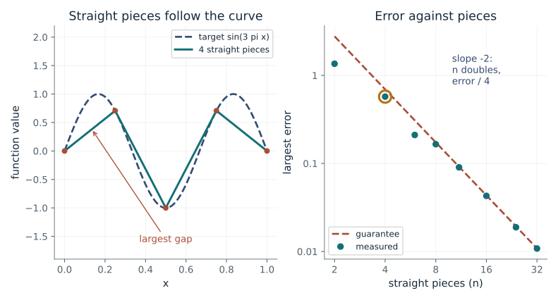
How can straight pieces joined at bends copy a smooth sine wave, and how fast does the gap close as you add pieces?

A bend changes the slope of the curve only after its position. Adding the slope changes to the first slope rebuilds the straight-piece copy of the sine exactly at the knots. Between knots the gap is controlled by how curved the target is.

Predict first: If you double the number of pieces from 4 to 8, by what factor does the guaranteed error shrink?

Straight pieces (n): 4

232

Left: sine curve with a 4-piece straight copy and its largest gap marked. Right: error against pieces on log axes, slope -2. — **Doubling the number of straight pieces cuts the worst-case error by four, because error scales like 1/n squared.**
Straight pieces (n): 4

With 4 pieces the largest error found is 0.574, under the guarantee 0.694. The guarantee falls fourfold each time n doubles, here to 0.173 at 8 pieces.

Largest error found: 0.574
Guaranteed upper bound: 0.694
Hinge neurons (bends): 3
Neurons with the linear term: 4

Why it matters for language models

This is the simplest case of why wider ReLU layers fit smooth functions better: each added neuron adds one bend. The 1/n^2 rate is the baseline against which deeper constructions are judged.

Show the calculation

Slopes come from differences of sin(3 pi x) at knots spaced 1/4. First slope = (sin(3 pi/4) - 0)/(1/4) = 2.83. Guarantee = (3 pi)^2 / (8 x 4^2) = 88.8 / 128 = 0.694. Count: 3 bends plus the linear term on [0,1] is 4 ReLUs. In general N ReLU neurons give at most N+1 linear pieces, so 4 pieces need at least 3 neurons.

The equations and symbols

$p_n(x)=s_0x+\sum_{j=1}^{n-1}(s_j-s_{j-1})\operatorname{ReLU}(x-j/n)$

$\|f-p_n\|_\infty\leq \|f^{\prime\prime}\|_\infty/(8n^2)$

n: number of straight pieces
s_j: slope of piece j
ReLU(z): z if z is positive, otherwise 0; it makes a bend
f: the target curve sin(3 pi x) on 0 to 1

Where the conclusion applies

Uniform knots and a twice continuously differentiable target. The maximum is sampled on 2001 points; the analytic bound is a supremum bound. N ReLU neurons give at most N+1 pieces.

Check your understanding: For n=4 pieces, how many bends and how many ReLUs in total build this copy on [0,1]?

Three bends plus one ReLU for the starting slope, four in total. Counting pieces as bends would miss the first slope.

Book source: Chapter 2, Approximating a Smooth Function with a Shallow ReLU Network. Illustration C02-D01. Illustration. Book sine target and hinge representation, with the linear term counted explicitly as one ReLU on [0,1]. Uses the sharper standard C2 interpolation bound (3 pi)^2/(8 n^2); the book states the looser (3 pi)^2/(2 n^2) with n-1 hidden neurons, so the companion bound is four times smaller. At 11 pieces (10 neurons) the sharper bound is 0.0918, matching the book numerical estimate of about 0.09. Sampled errors are recomputed. v39 EPUB / v43 print.

02 / 08

Folding multiplies pieces

From Chapter 2, The Triangle Wave Construction

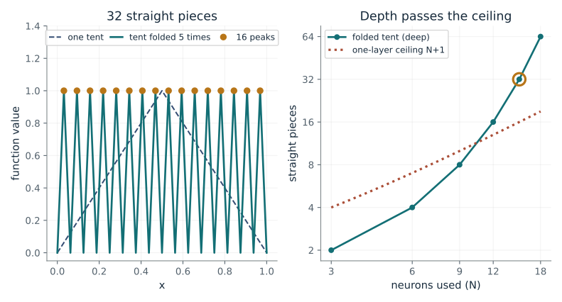
How many straight pieces does repeated folding create, and how does that compare with one wide layer?

Folding the interval in half and applying the tent again makes every existing piece into two. This proves efficient representation of this particular structured function, without proving efficient approximation of all functions.

Predict first: After four folds, are there sixteen peaks or sixteen pieces?

Folds (depth L): 5

16

Left: tent folded five times with 16 gold peaks. Right: pieces against neurons; folded tent curve rises above the one-layer N+1 line. — **Each fold doubles the pieces while adding a fixed three neurons, so depth overtakes any single wide layer after a few folds.**
Folds (depth L): 5

Folding 5 times gives 32 pieces from 15 neurons; one hidden layer of 15 neurons tops out at 16, so the tent is beyond that ceiling. Each fold doubles the pieces but adds only three neurons.

Straight pieces: 32
Peaks: 16
Neurons in the construction: 15
Most pieces one layer could give: 16

Why it matters for language models

Deep networks can represent very oscillatory functions with few parameters, which is one reason depth helps expressivity. It does not show that training will find such a network, or that arbitrary targets are cheap.

Show the calculation

Depth 5: 2^5 = 32 pieces and 2^4 = 16 peaks (each peak has two sides). Neurons: 3 x 5 = 15. A single hidden layer of N neurons has at most N+1 pieces, so 15 neurons allow 16. To match 32 pieces a single layer needs at least 31 neurons.

The equations and symbols

$T(x)=2\operatorname{ReLU}(x)-4\operatorname{ReLU}(x-1/2)+2\operatorname{ReLU}(x-1)$

$T^{\circ L}:\quad 2^L\text{ pieces},\quad 2^{L-1}\text{ peaks},\quad 3L\text{ neurons}$

T: the tent: rises from 0 to 1 then falls back to 0 on [0,1]
L: depth: how many times the tent is applied
N: neurons used; one hidden layer gives at most N+1 pieces

Where the conclusion applies

Only [0,1] is counted. A peak has two linear sides. Book Delta_k corresponds to L=k+1. The ceiling N+1 applies to one hidden layer with scalar input. This tent costs 3 neurons per fold (the book form); demo D07 builds a zigzag with 2 neurons per layer, so its counts differ. Both constructions are valid.

Check your understanding: Can every function of x be written as an outer function applied to T(x)?

No. T(x) = T(1-x), so any outer function gives the same value at x and 1-x. An asymmetric target cannot be copied this way.

Book source: Chapter 2, The Triangle Wave Construction. Illustration C02-D02. Illustration. Book statement; target functions, constants and seeds are companion illustrations. Counting note: the book says N ReLU neurons give at most N+1 linear pieces, so 2^k pieces need at least 2^k - 1 neurons in one layer. Exactly the normalized book tent; the 3L neuron count follows the book (the third term is zero on [0,1]). v39 EPUB / v43 print.

03 / 08

Why dimension is expensive

From Chapter 2, The Deep ReLU Network Achieves the Rate

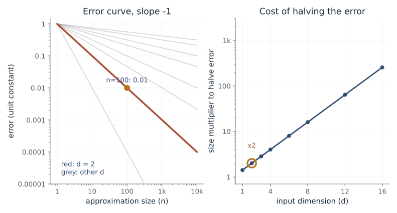
When the input has more dimensions, how much extra size does a smooth-function guarantee demand?

The rate n^(-s/d) divides smoothness by dimension. A function with many inputs needs exponentially more parameters to reach the same accuracy unless it has extra structure. Constants can hide additional dimension dependence.

Predict first: At fixed smoothness, will raising the dimension from 2 to 16 steepen or flatten the error curve?

Input dimension (d): 2

116

Smoothness (s)

Left: error against size on log axes, selected dimension in red over grey others. Right: size multiplier to halve error rising with dimension. — **The error exponent is smoothness divided by dimension, so each added dimension flattens the curve and makes every improvement costlier.**
Input dimension (d): 2 · Smoothness (s): 2

At smoothness s=2 and dimension d=2 the error falls like n^(-1). Halving the error needs 2 times more parameters; higher d flattens the curve and makes every gain costlier.

Error exponent (s/d): 1
Error at n = 100: 0.01
Size multiplier to halve the error: 2
Size multiplier for 10 times smaller: 10

Why it matters for language models

Language-model inputs are very high-dimensional, so smoothness alone cannot explain good performance; this is why structure and low-dimensional data patterns matter.

Show the calculation

Error = n^(-s/d) = n^(-2/2) = n^(-1). At n = 100: 100^(-1) = 0.01. To halve the error multiply n by 2^(d/s) = 2^(2/2) = 2. To cut it tenfold multiply n by 10^(d/s) = 10. Constants are set to one.

The equations and symbols

$\text{error}(n)\propto n^{-s/d}$

$\text{size multiplier to halve the error}=2^{d/s}$

n: approximation size (parameters)
s: smoothness: how many derivatives the target has
d: input dimension: number of input variables

Where the conclusion applies

Sobolev-type statement with bounded smoothness norm; constants and logarithmic factors are set to one, so only the exponent is meaningful.

Check your understanding: For s=2, d=4, what size multiplier halves the error?

Four: the exponent is 1/2, so multiplying n by four multiplies error by 4^(-1/2) = 1/2.

Book source: Chapter 2, The Deep ReLU Network Achieves the Rate. Illustration C02-D03. Illustration. Book principle; unit constants are companion illustrations. v39 EPUB / v43 print.

04 / 08

Three different reasons for failure

From Chapter 2, Width vs. Depth: The Modern Picture

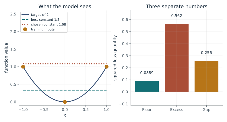
When a fitted model misses, is the cause the model family, the optimizer, or the sample?

The floor is what the family cannot represent. The chosen constant adds a separate optimization excess. Training locations change the training risk and so the signed sample gap, not the exact floor.

Predict first: Can the sample gap (population risk minus training risk) become negative?

Offset from best constant: 0.75

01

Training locations

Left: x squared with a best constant, a chosen constant and gold training points. Right: three bars for floor, excess and signed sample gap. — **The floor, the optimizer excess and the sample gap are three separate numbers; fixing one does not fix the others.**
Offset from best constant: 0.75 · Training locations: balanced

Floor (representation) is fixed at 0.0889; the chosen constant adds excess 0.562 from optimization. The sample gap is 0.256 (positive: training looks better than the population).

Population risk: 0.651
Risk on training inputs: 0.396
Floor (best constant): 0.0889
Signed sample gap: 0.256

Why it matters for language models

A training loss can look better or worse than held-out loss depending on where the training examples sit, so a validation gap needs a look at the data before blaming the model.

Show the calculation

E[x^2] = 1/3 and E[x^4] = 1/5, so the best constant has risk 1/5 - 1/9 = 4/45 = 0.0889. Moving to c = 1/3 + 0.75 = 1.08 adds 0.75^2 = 0.562, so population risk = 0.651. On the training inputs, mean of (x^2 - c)^2 = 0.396. Gap = 0.651 - 0.396 = 0.256.

The equations and symbols

$R(c)=\mathbb E_{x\sim U[-1,1]}(x^2-c)^2=4/45+(c-1/3)^2$

$\text{Signed sample gap}=R(c)-\widehat R(c)$

R: population risk: average squared error over all x in [-1,1]
R-hat: average squared error on the training inputs only
c: the constant the model predicts, 1/3 plus the offset
offset: how far the optimizer stopped from the best constant

Where the conclusion applies

Constant hypothesis family, noiseless target, uniform population. The best constant is population-best, not assumed to be empirical-best. At offset 0.5 with the balanced sample the floor 4/45 and the sample gap coincide numerically; they remain different quantities.

Check your understanding: If the offset is zero, does a constant represent x squared exactly?

No. Optimization excess becomes zero but the floor 4/45 stays, because no constant equals x squared across the population.

Book source: Chapter 2, Width vs. Depth: The Modern Picture. Illustration C02-D04. Illustration. Book principle; explicitly specified toy inputs and constants are companion illustrations. v39 EPUB / v43 print.

05 / 08

Random cosines copy a kernel

From Chapter 2, The Test of Time (random Fourier features)

How many random cosine features does it take to copy a smooth similarity score closely?

Each random cosine pair gives an unbiased but noisy estimate of the similarity. Averaging D independent estimates shrinks the spread by the square root of D, the same law as repeated coin flips.

Predict first: If you make D four times larger, what happens to the typical error?

Random features (D): 16

4512

Distance between points (r)

Left: exact Gaussian kernel and a dashed copy from 16 random cosines. Right: error against D on log axes, falling with slope -1/2. — **The error of random features falls like 1 over the square root of D, so quadrupling the features only halves the error.**
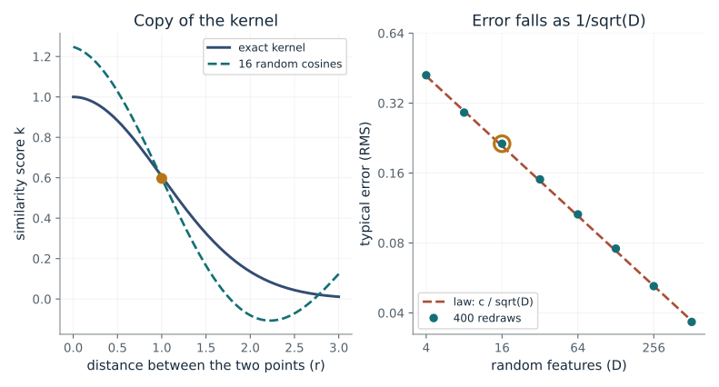
Random features (D): 16 · Distance between points (r): 1

At distance 1 the exact score is 0.607; one draw of 16 cosines gives 0.597. Across 400 redraws the typical error is 0.214, close to the 0.209 the 1/sqrt(D) law predicts.

Exact similarity: 0.607
Estimate from these D features: 0.597
Typical error at D = 16: 0.214
Law: typical error at 4 times D: 0.105

Why it matters for language models

Random feature maps are used to approximate attention-style similarity scores at lower cost. This rate shows the price: each extra digit of accuracy needs a hundred times more features.

Show the calculation

One feature product has mean k = exp(-r^2/2) = 0.607 and variance 1 + exp(-2r^2)/2 - exp(-r^2) = 0.7. Averaging D independent products divides the variance by D, so the typical error is sqrt(0.7/16) = 0.209. With 4D features it is half of that: 0.105. The measured value 0.214 comes from seeded redraws.

The equations and symbols

$z_D(x)=\sqrt{2/D}\,\big(\cos(\omega_1^\top x+b_1),\ldots,\cos(\omega_D^\top x+b_D)\big)$

$z_D(x)^\top z_D(y)\approx k(x,y)=e^{-\|x-y\|^2/2},\quad \text{typical error}=\sqrt{\mathrm{Var}/D}$

D: number of random cosine features
omega: random frequency, drawn from a standard normal
b: random phase, uniform from 0 to 2 pi
k: similarity score between two points
r: distance between the two points

Where the conclusion applies

Unit-width Gaussian kernel and one pair of points per panel. Typical error is the root mean square over 400 seeded redraws. The book uniform guarantee over all pairs adds logarithmic factors that this one-pair picture omits.

Check your understanding: To make the typical error ten times smaller, how much larger must D be?

One hundred times larger, because error is proportional to D^(-1/2) and 100^(-1/2) = 1/10.

Book source: Chapter 2, The Test of Time (random Fourier features). Illustration C02-D05. Illustration. Book random Fourier feature construction (Rahimi and Recht); Gaussian kernel, two-dimensional inputs and seeds (11 and 5) are companion illustrations. v39 EPUB / v43 print.

06 / 08

When dimension-free beats dimension-hungry

From Chapter 2, The Dimension Problem in Practice

The Barron rate ignores dimension but carries a constant. At what input dimension, and from what size, does it beat the smoothness rate?

The Barron error falls like n^(-1/2) at every dimension, while the Sobolev error falls like n^(-s/d). Once s/d drops below 1/2 the first curve eventually undercuts the second. The Barron norm C shifts where that happens.

Predict first: At smoothness 2, from which input dimension does the dimension-free rate win at large n?

Input dimension (d): 4

232

Barron norm (C)

Left: Barron and Sobolev error curves at d=4, parallel lines. Right: crossover size against dimension, shaded below d=4 where Sobolev never loses. — **The Barron rate wins only when the dimension is more than twice the smoothness, and a large Barron norm delays that win enormously.**
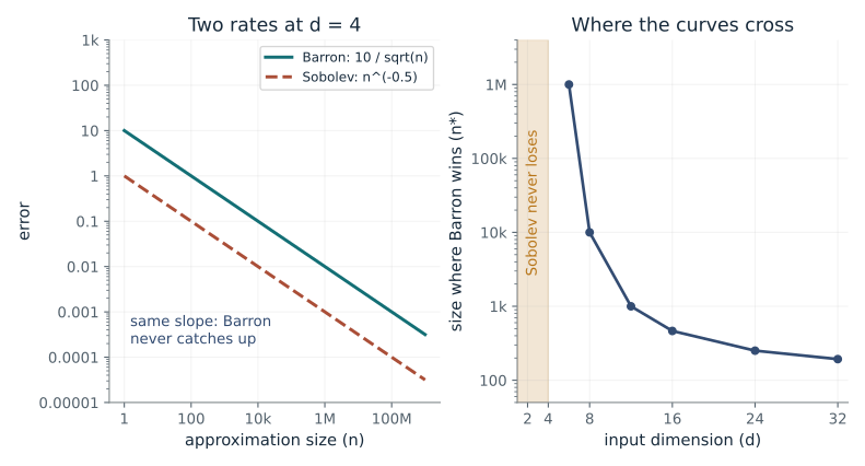
Input dimension (d): 4 · Barron norm (C): 10

At d=4 the Sobolev exponent 0.5 is at least the Barron exponent 0.5, so the two curves never cross in favour of Barron. Dimension-free does not mean better in low dimension.

Barron exponent: 0.5
Sobolev exponent (2/d): 0.5
Crossover size n*: undefined (Sobolev rate is at least as fast)
Error at the crossover: undefined

Why it matters for language models

It explains why networks can beat grid-like methods on high-dimensional inputs, and why that depends on the target being of a particular, narrower type rather than on dimension alone.

Show the calculation

Barron error = 10 n^(-1/2). Sobolev error = n^(-2/4) = n^(-0.5). Exponent gap = 1/2 - 2/4 = 0, which is not positive, so Barron never overtakes for a Barron norm of 10 or more.

The equations and symbols

$\text{Barron: } C/\sqrt{n},\qquad \text{Sobolev: } n^{-s/d}$

$C n^{-1/2}=n^{-s/d}\;\Rightarrow\; n^*=C^{1/(1/2-s/d)}\quad(d>2s)$

C: Barron norm: how wiggly the target is in frequency terms
n: approximation size
s: smoothness, fixed at 2 here
d: input dimension
n*: size beyond which Barron is the smaller error

Where the conclusion applies

Smoothness s = 2; Barron norm C at least 1; the target must satisfy both assumptions to compare. If d <= 2s the Sobolev exponent is at least 1/2 and no crossover exists.

Check your understanding: At d = 8 and s = 2, with C = 100, what size n* does the crossover need?

The exponent gap is 1/2 - 1/4 = 1/4, so n* = 100^4 = 10^8: the dimension-free rate wins only at very large sizes.

Book source: Chapter 2, The Dimension Problem in Practice. Illustration C02-D06. Illustration. Book rates C/sqrt(n) (as the root of the squared-error rate C^2/n) and n^(-s/d); the constants C and the unit Sobolev constant are companion illustrations. The two rates need different target assumptions and norms, so this is a comparison of exponents and constants, not one certified error. v39 EPUB / v43 print.

07 / 08

Depth multiplies, width adds

From Chapter 2, Width, Depth, and the Minimal Network (Lemma 2.3, linear regions)

For the same number of neurons, how many straight pieces can stacked layers make compared with one wide layer?

A layer that folds the interval m times turns each existing piece into m pieces. Repeating the layer L times multiplies the pieces by m each time, while the neurons only add. A single layer cannot multiply: N neurons give at most N+1 pieces.

Predict first: If the depth doubles from 3 to 6 layers of 3 neurons, how do the neuron count and the piece count change?

Layers (depth L): 3

16

Neurons per layer (m)

Left: zigzag output of a 3-layer network, 27 pieces. Right: pieces against depth for the built network, the book bound and one layer. — **Neurons add up across layers but pieces multiply, so the same neuron budget gives far more pieces when stacked.**
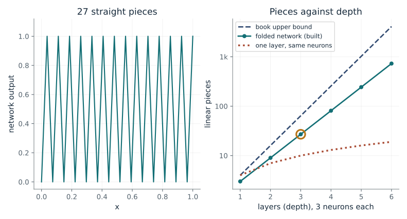
Layers (depth L): 3 · Neurons per layer (m): 3

9 neurons arranged in 3 layers of 3 give 27 pieces. Put in one layer they could give at most 10. Each extra layer multiplies the count by 3 instead of adding 3.

Neurons in total: 9
Linear pieces counted: 27
Most one layer of that size gives: 10
Upper bound from the book: 64

Why it matters for language models

This is one concrete reason deep networks can carve input space far more finely than wide shallow ones. The count is a ceiling on flexibility, not evidence that training will use it.

Show the calculation

Each layer folds [0,1] into 3 full-height zigzags (cost 3 neurons). Pieces multiply: 3^3 = 27. Neurons add: 3 x 3 = 9. One hidden layer of N neurons has at most N+1 = 10 pieces. The book bound for one input is (m+1)^L = 4^3 = 64, and 27 <= 64.

The equations and symbols

$\text{one layer, }N\text{ neurons: at most }N+1\text{ pieces}$

$\text{width }m,\ \text{depth }L:\quad m^L\text{ pieces built},\ \le (m+1)^L\text{ allowed (1-D input)}$

m: neurons per layer (width)
L: number of layers (depth)
N: total neurons, m times L

Where the conclusion applies

Scalar input on [0,1]. Each layer is a zigzag with m full-height pieces built from m ReLUs (so a tent is 2 neurons here, versus 3 per fold in D02; both are valid). Pieces are counted numerically from bends on a grid containing every breakpoint. The upper bound requires width at least the input dimension.

Check your understanding: How many neurons does one hidden layer need to produce 64 pieces, and how many does the folded tent need?

At least 63 neurons in one layer. The tent with 6 folds uses 3 x 6 = 18 neurons.

Book source: Chapter 2, Width, Depth, and the Minimal Network (Lemma 2.3, linear regions). Illustration C02-D07. Illustration. Book statement; target functions, constants and seeds are companion illustrations. Counting note: the book says N ReLU neurons give at most N+1 linear pieces, so 2^k pieces need at least 2^k - 1 neurons in one layer. The zigzag network is a companion construction; the upper bound is the book Lemma 2.3 (Montufar et al., 2014) with input dimension 1. v39 EPUB / v43 print.

08 / 08

Finer grid, faster shrinking error

From Chapter 2, The Superposition Revisited: KANs (Theorem 2.13a)

In a spline network the learnable curves live on a grid. How fast does the error fall as the grid is refined?

A smooth curve looks almost like a polynomial over a short interval. Cubic pieces match the curve far better than straight ones on the same grid, so shrinking the intervals helps much faster.

Predict first: Does using smoother spline pieces change how quickly the error falls as the grid is refined?

Grid intervals (G): 8

432

Spline order (k)

Left: sine curve with an 8-interval straight-piece fit. Right: error against grid size for orders 1, 2, 3 on log axes with the selected point circled. — **Spline order sets the slope on the log plot: order k gives error proportional to G to the power minus (k+1).**
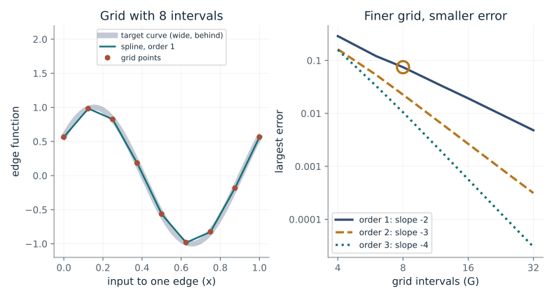
Grid intervals (G): 8 · Spline order (k): 1

An order-1 spline on 8 intervals is off by at most 0.0745. Doubling the grid shrinks that by 3.88, close to the predicted 4: smoother pieces make refinement pay more.

Largest error: 0.0745
Error with 16 intervals: 0.0192
Observed shrink factor: 3.88
Predicted factor 2^(k+1): 4

Why it matters for language models

Learnable-spline layers trade parameters (grid size) for accuracy; the order of the spline decides how much each extra grid point buys.

Show the calculation

Theory: error ~ G^-(k+1) = G^-2. Doubling G divides the error by 2^2 = 4. Measured here: 0.0745 / 0.0192 = 3.88. Target is sin(2 pi x + 0.6), one smooth edge function; the constant in the bound depends on the target.

The equations and symbols

$\|f-f_{\mathrm{KAN}}\|_\infty\leq C_{k,d}\,G^{-(k+1)}$

$\text{error ratio when }G\to 2G:\ 2^{k+1}$

G: number of grid intervals on each edge curve
k: spline order: 1 is straight pieces, 3 is cubic
C: constant depending on the target and the dimension

Where the conclusion applies

One univariate edge function fitted by interpolation at the grid points, not a full KAN. The theorem needs a smooth Kolmogorov-type decomposition; cubic fits need at least 4 intervals.

Check your understanding: With cubic pieces, by what factor does the error shrink when the grid goes from 8 to 16 intervals?

About 16, since 2^(3+1) = 16. For this sine the measured ratio at 8 intervals is 18.6: it is not exactly 16 because the grid is still coarse. It wanders (15.1, 18.6, 18.8, 17.8 from 4 to 32 intervals) and settles toward 16 as the grid gets finer.

Book source: Chapter 2, The Superposition Revisited: KANs (Theorem 2.13a). Illustration C02-D08. Illustration. Book Theorem 2.13a rate G^-(k+1) for one spline edge; the target sin(2 pi x + 0.6) and interpolation at the grid points are companion illustrations. v39 EPUB / v43 print.

Build a curve from bends

Folding multiplies pieces

Why dimension is expensive

Three different reasons for failure

Random cosines copy a kernel

When dimension-free beats dimension-hungry

Depth multiplies, width adds

Finer grid, faster shrinking error

Bring the idea to a question of your own