Chapter 3 · Optimization and Training Dynamics

01 / 08

Where a step size stops working

From Chapter 3, The Double-Well: A Nonconvex Landscape in One Dimension

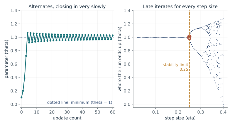
You walk downhill in a double-well landscape. How large can the step be before the walk stops settling on the bottom, and what happens just past that limit?

Each update subtracts the step size times the slope. Right at the bottom the slope changes at rate 8, so an error is multiplied by 1 - 8 eta each update. Below 0.25 that factor is smaller than 1 in size and errors die out; above 0.25 it is larger than 1 in size and the bottom repels the walk.

Predict first: At the stability limit 0.25 the walk keeps flipping from one side of the bottom to the other. Does a lasting two-point cycle form right there, or only at a larger step?

Step size (eta): 0.25

0.050.35

Left: walk in a double well, flipping around the minimum at 1. Right: late positions for every step size, splitting into branches past 0.25. — **Past the step limit the bottom stops being stable, but a curved loss can trap the walk in a repeating cycle instead of sending it to infinity.**
Step size (eta): 0.25

At exactly the limit the error rule is -1, so the run keeps flipping from one side of 1 to the other. The curve of the well pulls it in, but only very slowly (about 0.005 away after 3000 updates). No lasting two-cycle forms here.

Error rule near the minimum (1 - 8 x eta): -1
First update: 0.199
After 60 updates: 1.03
Long-run behaviour: alternates, closing in slowly

Why it matters for language models

Choosing a learning rate that is too large makes training loss bounce instead of settle. Real losses are not parabolas, so the bounce can persist as a cycle or wander rather than blow up.

Show the calculation

First update: theta_1 = 0.1 - 0.25 x 4(0.1)(0.1^2 - 1) = 0.1 + 0.25 x 0.396 = 0.199. The well bottom has curvature F''(1) = 12 - 4 = 8, so the stability limit is 2/8 = 0.25. Error rule near theta = 1: 1 - 8 x 0.25 = -1. A start of exactly 0 never moves, because the slope there is 0.

The equations and symbols

$\theta_{t+1}=\theta_t-\eta F^{\prime}(\theta_t)$

$F(\theta)=(\theta^2-1)^2,\quad F^{\prime}(\theta)=4\theta(\theta^2-1),\quad F^{\prime\prime}(\pm1)=8$

$\text{error near the bottom: }\ e_{t+1}=(1-8\eta)\,e_t$

theta: the single number being adjusted (the parameter)
eta: step size: how far each update moves
F: the loss; its two bottoms are at theta = 1 and theta = -1
1 - 8 eta: factor by which the distance to the bottom changes each update

Where the conclusion applies

Exact gradients, start 0.1, 60 updates drawn and 4000 used to classify the long run. A start of exactly 0 is the maximum of the well and never moves. The stability limit 2/8 = 0.25 is a local rule near the bottom, not a guarantee of convergence from every start.

Check your understanding: Take the wider well F = (theta^2 - 4)^2, whose bottoms are at theta = 2 and -2. What is its step-size limit?

The curvature at the bottom is 12 x 4 - 16 = 32, so the limit is 2/32 = 0.0625. A wider, steeper well needs a much smaller step.

Book source: Chapter 3, The Double-Well: A Nonconvex Landscape in One Dimension. Illustration C03-D01. Illustration. Book double well and its start at 0.1. Uses the corrected book text: at eta = 0.25 the iterates alternate and close in very slowly, and a lasting two-cycle (0.731, 1.14) appears at eta = 0.3. v39 EPUB / v43 print.

02 / 08

Noisy evidence and averaging

From Chapter 3, The Noise That Helps

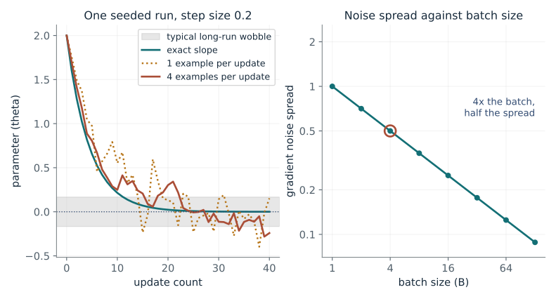
Each training example gives a noisy reading of the slope. How much noise does averaging a batch of them remove?

Independent errors partly cancel when averaged. Their variances add, so the sum of B readings has variance B times sigma squared; dividing the sum by B divides that variance by B squared, leaving sigma squared over B. The parameter then moves by step size times that error, so the wobble around the best value scales with the same spread.

Predict first: If the batch size is multiplied by four, does the noise variance or the noise spread (standard deviation) get cut in half?

Batch size (B): 4

1128

Noise of one example (sigma)

Left: exact and noisy runs of a parameter settling near zero inside a grey band. Right: noise spread falling with batch size on log axes. — **Averaging B independent readings divides the noise variance by B, so the spread falls only as 1 over the square root of B.**
Batch size (B): 4 · Noise of one example (sigma): 1

Averaging 4 examples cuts the noise variance to 0.25, so the spread is 0.5. The run settles near zero and wobbles by about 0.167. Quadrupling the batch halves the spread; it quarters the variance.

Gradient noise variance (sigma^2 / B): 0.25
Gradient noise spread (square root of that): 0.5
Long-run wobble of theta: 0.167
Final theta in this run: -0.241

Why it matters for language models

Language-model training averages gradients over many tokens per step. Each fourfold increase in batch only halves the gradient noise, which is why very large batches give diminishing returns.

Show the calculation

One example has variance 1^2 = 1. Averaging 4: 1/4 = 0.25; spread = square root = 0.5. Each update shifts theta by eta x error = 0.2 x error, so the long-run wobble is sqrt(0.2 x 0.25/1.8) = 0.167. First update in this run: 2 - 0.2(2 - 0.463) = 1.693.

The equations and symbols

$\widehat g_B=B^{-1}\sum_{i=1}^{B}g_i$

$\operatorname{Var}(\widehat g_B)=\sigma^2/B,\qquad \operatorname{sd}(\widehat g_B)=\sigma/\sqrt{B}$

B: batch size: examples averaged per update
sigma: spread (standard deviation) of the noise from one example
eta: step size, fixed at 0.2 here
theta: the parameter; the true loss is theta^2/2, so the best value is 0

Where the conclusion applies

Independent zero-mean Gaussian noise, one seeded run of 40 updates (seed 303). No finite-population correction. Dependent examples need covariance terms, so the 1/B rule does not hold for them.

Check your understanding: Two noise readings each have variance 1 but are correlated, with covariance 0.5. What is the variance of their average?

(1 + 1 + 2 x 0.5)/4 = 0.75, larger than the independent value 0.5. Correlation limits how much averaging helps.

Book source: Chapter 3, The Noise That Helps. Illustration C03-D02. Derived specialization. Book principle; the toy loss, step size 0.2 and seed 303 are companion choices. v39 EPUB / v43 print.

03 / 08

Remembering past changes

From Chapter 3, The Algorithm That Remembers

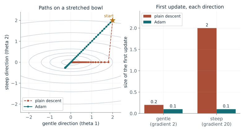
Adam keeps running averages of the gradient and of its square. What does that do to the very first update?

Adam tracks the average gradient and the average squared gradient separately. At the start both averages are shrunk toward their zero start, so each is divided by one minus its memory factor to undo that. Dividing the direction by the square root of the squared average makes the first update about the step size in every coordinate.

Predict first: The gradient in the steep (second) coordinate is ten times the gradient in the gentle (first) coordinate. Is Adam's first update ten times larger in the steep coordinate?

Memory of the gradient (beta1)

Step size (eta): 0.1

0.020.15

Left: Adam and plain descent paths on a stretched bowl from a start at (2, 2). Right: bars of first update size per direction. — **Adam rescales every coordinate by its own recent gradient size, so a direction with a huge gradient does not get a huge first update.**
Memory of the gradient (beta1): 0.9 · Step size (eta): 0.1

The steep direction has a gradient ten times larger, so plain descent moves it ten times farther on the first update. Adam divides each direction by its own recent gradient size, so both first updates are about eta = 0.1.

First gradient: (2, 20)
First Adam update (sizes): (0.1, 0.1)
First plain update (sizes): (0.2, 2)
Objective after 40 updates, Adam / plain: 0.309 / 0.000437

Why it matters for language models

Language-model parameters have gradients of very different sizes (embeddings against attention weights). Per-coordinate rescaling keeps every parameter moving at a comparable rate.

Show the calculation

First gradient (2, 20). m1 = (1 - 0.9) x (2, 20) = (0.2, 2); v1 = 0.01 x (4, 400) = (0.04, 4). Bias correction divides by 1 - 0.9 and by 0.01, giving back (2, 20) and (4, 400). Update = 0.1 x 2 / sqrt(4) = 0.1 and 0.1 x 20 / sqrt(400) = 0.1. Plain descent: 0.1 x (2, 20) = (0.2, 2).

The equations and symbols

$m_t=\beta_1m_{t-1}+(1-\beta_1)g_t,\quad v_t=\beta_2v_{t-1}+(1-\beta_2)g_t^2$

$\widehat m_t=m_t/(1-\beta_1^t),\quad\widehat v_t=v_t/(1-\beta_2^t)$

$\theta_t=\theta_{t-1}-\eta\,\widehat m_t/(\sqrt{\widehat v_t}+\epsilon)$

m: running average of the gradient (its direction)
v: running average of the squared gradient (its size)
beta1: memory of m; 0 means no memory (set by the control)
eta: step size
epsilon: tiny number 1e-8 that avoids dividing by zero

Where the conclusion applies

m0 = v0 = 0, t starts at 1, 0 <= beta1 < 1. Exact gradients of (theta1^2 + 10 theta2^2)/2, 40 updates. Squares and divisions act on each coordinate separately. A fixed toy run, no claim that Adam beats plain descent in general.

Check your understanding: The gradient is a constant 3 and beta1 = 0.5. What are m after two updates and its bias-corrected value?

m1 = 1.5, m2 = 0.5 x 1.5 + 0.5 x 3 = 2.25. Corrected: 2.25/(1 - 0.25) = 3. The correction removes the shrinkage from starting at zero.

Book source: Chapter 3, The Algorithm That Remembers. Illustration C03-D03. Illustration. Book equations; the stretched bowl (curvatures 1 and 10), start (2, 2), beta2 = 0.99 and epsilon = 1e-8 are companion choices. v39 EPUB / v43 print.

04 / 08

Large steps early, small steps later

From Chapter 3, The Shape of the Schedule; The Continuous-Time Limit

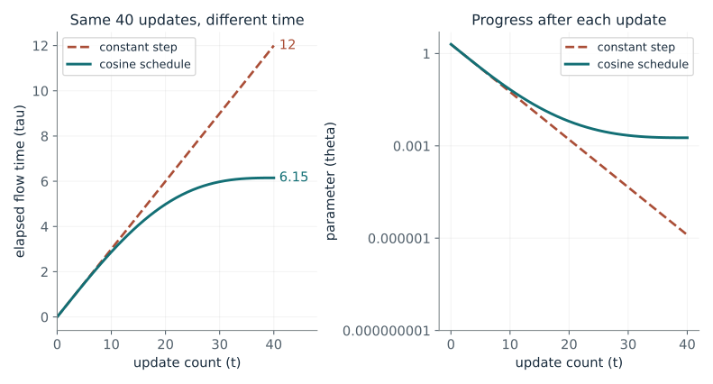
A schedule shrinks the step size over training. Does making the same number of updates mean covering the same distance along the smooth downhill flow?

The smooth flow is the limit of infinitely many tiny steps. A run of steps of size eta_t has travelled for a flow time equal to the sum of those sizes, so a schedule that shrinks its steps covers less time in the same number of updates. Late small steps trade speed for fine control.

Predict first: Both runs make 40 updates. Do they cover the same elapsed flow time?

Largest step size: 0.3

0.10.6

Smallest step size

Left: elapsed flow time against update count, constant steps above a flattening cosine schedule. Right: parameter against updates on a log axis. — **Equal update counts are not equal distances: a shrinking schedule covers less flow time, so it makes less progress per update than a constant step of the same size.**
Largest step size: 0.3 · Smallest step size: 0

Both runs make 40 updates, but the cosine schedule only covers 6.15 units of flow time while the constant step covers 12. It has made less progress: theta shrank by 3.04 powers of ten, against 6.2 for the constant step.

Elapsed time, constant step: 12
Elapsed time, cosine schedule: 6.15
Step size at update 20: 0.15
Powers of ten shrunk after 40 updates, cosine / constant: 3.04 / 6.2

Why it matters for language models

Language-model training usually decays the learning rate (often with a cosine shape) after a warm-up. Comparing runs fairly means comparing total step size, not just the number of updates.

Show the calculation

Halfway, cos(pi/2) = 0, so the step size is (0.3 + 0)/2 = 0.15. Constant: elapsed time = 40 x 0.3 = 12. Cosine: add up all 40 step sizes = 6.15. First update from 2: Euler gives 2(1 - 0.3) = 1.4; the smooth flow gives 2 exp(-0.3) = 1.48.

The equations and symbols

$\eta_t=\eta_{\min}+\tfrac12(\eta_{\max}-\eta_{\min})(1+\cos(\pi t/T))$

$\dot\theta=-\theta,\quad\theta(\tau)=2e^{-\tau}$

t: update count, from 0 to T = 40
eta_max, eta_min: largest and smallest step size of the cosine schedule
tau: elapsed flow time: the sum of all step sizes so far
theta: the parameter; the loss is theta^2/2, starting at 2

Where the conclusion applies

0 <= minimum <= maximum. Each update is one Euler step whose size is the step size, so the elapsed flow time is the running sum of step sizes. The smooth flow theta = 2 exp(-tau) is shown only in the worked arithmetic. Not a claim that a lower endpoint gives a better solution.

Check your understanding: A cosine schedule falls from 0.4 to 0 over 100 updates. What step size does it use at update 50 and at update 100?

At update 50 the cosine term is 0, so the step is 0.4/2 = 0.2. At update 100 it reaches 0, but that final value is not used for an update.

Book source: Chapter 3, The Shape of the Schedule; The Continuous-Time Limit. Illustration C03-D04. Illustration. Book schedule and flow equations; the toy loss, T = 40 and the starting value 2 are companion choices. v39 EPUB / v43 print.

05 / 08

Past the edge, a curved loss pulls itself back

From Chapter 3, When Sharpness Grows Until It Cannot Grow Further

On a parabola, gradient descent blows up once the curvature (sharpness) exceeds 2 divided by the step size. Must that also happen on a loss that curves more steeply away from its bottom?

Each update multiplies theta by 1 - eta lambda - eta mu theta^2. Away from zero the last term makes the factor smaller in size than the parabola's, so the bounces shrink. As theta shrinks, the sharpness 1 + 3 theta^2 falls toward its floor. If the floor is only just below 2/eta, shrinking is slow and the sharpness lingers at the edge.

Predict first: Start where the sharpness is above 2/eta. A parabola would blow up. Does the curved loss blow up too, and how long can it stay near the edge?

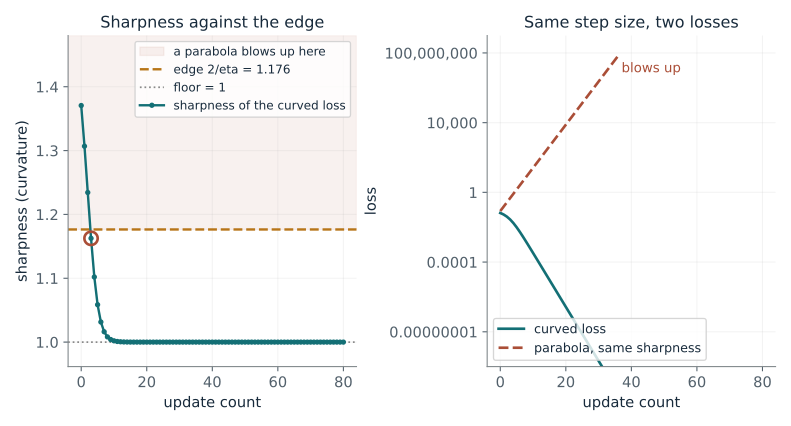
Step size (eta): 1.7

0.51.99

Left: sharpness against updates with the 2/eta edge line and floor of 1. Right: curved loss falling while a same-sharpness parabola blows up. — **A loss that flattens as the walk shrinks its bounces can survive past 2/eta, and the closer 2/eta is to the bottom curvature, the longer it hovers at the edge.**
Step size (eta): 1.7

The start is past the edge (sharpness 1.371 against 2/eta = 1.176). A parabola with that sharpness would blow up, but here every bounce is a little smaller than the last, so sharpness drops under the edge after 3 updates. The closer 2/eta is to the floor of 1, the longer it hovers there.

Edge of stability (2 / eta): 1.176
Starting sharpness: 1.371
Updates spent above the edge: 3
Sharpness after 80 updates: 1

Why it matters for language models

Full-batch training of neural networks is observed to sit with sharpness near 2 over the learning rate while the loss still falls. The simple parabola rule would have predicted divergence.

Show the calculation

Update: theta_next = theta x (1 - 1.7 - 1.7 theta^2). Start theta_0 = 0.3515, so sharpness = 1 + 3 x 0.124 = 1.371; edge = 2/1.7 = 1.176. Size of the first change: curved loss |1 - 1.7 - 1.7 x 0.124| = 0.910 (shrinks); parabola |1 - 1.7 x 1.371| = 1.330 (grows).

The equations and symbols

$F(\theta)=\tfrac{\lambda}{2}\theta^2+\tfrac{\mu}{4}\theta^4,\qquad F^{\prime\prime}(\theta)=\lambda+3\mu\theta^2$

$\theta_{t+1}=\theta_t\bigl(1-\eta\lambda-\eta\mu\theta_t^2\bigr)$

$\text{parabola: stable only if }F^{\prime\prime}<2/\eta$

sharpness: the curvature F''(theta) at the current point
2/eta: the edge of stability: the sharpness a parabola can tolerate
lambda: curvature at the very bottom (set to 1)
mu: how fast the curvature grows away from the bottom (set to 1)

Where the conclusion applies

Exact gradients, 80 updates, 0 < eta lambda < 2. The start is set inside the window where sharpness exceeds 2/eta but the curved update still shrinks. This toy shows only the self-correcting half of the edge-of-stability story; it does not show sharpness rising during training in a real network.

Check your understanding: With lambda = 1 and eta = 1.5, what is the edge 2/eta, and can sharpness settle at the floor value 1?

The edge is 2/1.5 = 1.33. The floor 1 is below it, so the bottom itself is stable and sharpness ends at 1. If instead eta were above 2, even the floor would sit past the edge and the walk could not settle.

Book source: Chapter 3, When Sharpness Grows Until It Cannot Grow Further. Illustration C03-D05. Illustration. Book worked example for the nonquadratic loss F = (lambda/2)theta^2 + (mu/4)theta^4. lambda = mu = 1 and the starting point are companion choices. v39 EPUB / v43 print.

06 / 08

How a stretched bowl slows descent

From Chapter 3, The Landscape Before the Walk

When a loss bowl is far steeper in one direction than another, how many updates does gradient descent need, and how does that grow as the bowl gets more stretched?

The steepest direction limits the step to 1/L. In the gentlest direction that step only removes a fraction mu/L of the error per update. A larger L over mu means a smaller fraction removed each time, so more updates are needed.

Predict first: If the bowl becomes ten times more stretched (condition number 10 to 100), do you need about ten times as many updates, or far more?

Condition number (kappa = L/mu): 10

2100

Step rule

Left: loss gap curves on a log axis for eight condition numbers, one highlighted. Right: updates needed rising with condition number. — **Under the PL guarantee the loss gap shrinks by 1 - mu/L per update, so the number of updates grows in proportion to the condition number.**
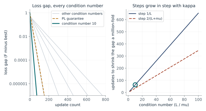
Condition number (kappa = L/mu): 10 · Step rule: step 1/L

With condition number 10, the loss gap needs 63 updates to shrink a million-fold. The PL guarantee allows for 132, and the real curve stays under it. A ten times more stretched bowl needs about ten times more updates.

Condition number (L / mu): 10
Guaranteed shrink per update (1 - mu/L): 0.9
Updates needed (million-fold smaller gap): 63
Updates the guarantee allows for: 132

Why it matters for language models

The condition number of the loss curvature is a main reason deep-network training is slow with plain gradient descent, and the reason adaptive and preconditioned methods are used.

Show the calculation

L = 1, mu = 1/10 = 0.1. Guaranteed shrink per update: 1 - mu/L = 0.9. Million-fold shrink needs T with 0.9^T <= 0.000001, so T >= ln(1,000,000) / (-ln 0.9) = 13.8 / 0.105 -> 132. The exact loop for this step 1/L reaches it after 63 updates.

The equations and symbols

$\tfrac12\|\nabla F\|^2\ge\mu\,(F-F^*)$

$F(\theta_T)-F^*\le\bigl(1-\tfrac{\mu}{L}\bigr)^T\,(F(\theta_0)-F^*)$

$\kappa=L/\mu$

mu: gentlest curvature; the PL constant
L: steepest curvature; sets the largest safe step 1/L
kappa: condition number L/mu: how stretched the bowl is
F - F*: loss gap: how far the loss is above its best value

Where the conclusion applies

Exact gradients of a two-direction quadratic, which satisfies the PL condition with constant mu. The guarantee is stated for the step 1/L; the step 2/(L+mu) is shown for comparison and also stays under the same curve here. 800 updates drawn; step counts are found by running the exact loop.

Check your understanding: A loss has L = 4 and mu = 0.1. By the guarantee, roughly how many updates give a million-fold smaller gap?

kappa = 40, so the shrink per update is 1 - 1/40 = 0.975. ln(1,000,000)/(-ln 0.975) = 13.8/0.0253, about 546 updates (an upper estimate; the real run is faster).

Book source: Chapter 3, The Landscape Before the Walk. Illustration C03-D06. Derived specialization. Book Theorem 3.1 (PL convergence). The two-direction quadratic F = (x^2/kappa + y^2)/2 with L = 1 and start (sqrt(kappa), 1) is a companion choice. v39 EPUB / v43 print.

07 / 08

Learning in stages

From Chapter 3, Linear Networks and the Bias That Lives in the Path

In a simple two-layer linear network, is every pattern in the data learned at the same pace, or does training learn the strongest patterns first?

The growth rate of a direction is proportional to its own current size, so a tiny start grows slowly and then explosively until it nears its target. A stronger direction (larger target) grows faster, so it escapes its flat start sooner.

Predict first: Shrink the starting strength by a factor of 10 (0.001 to 0.0001). Do the three directions get learned closer together in time, or further apart?

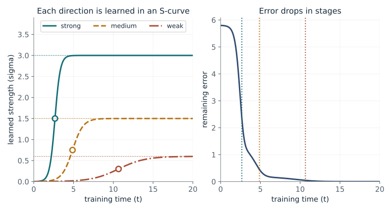
Starting strength (sigma at t = 0): 0.001

3e-050.1

Left: three S-shaped learning curves reaching targets 3, 1.5 and 0.6 at different times. Right: total error falling in stages. — **Each direction is learned along an S-curve, the strongest first, and a smaller start makes the waits longer and the stages sharper.**
Starting strength (sigma at t = 0): 0.001

Each direction follows an S-curve: nearly flat at first, then a quick rise, then a plateau at its target. The strong direction is half-learned at t = 2.67, the weak one not until t = 10.7. A smaller start makes the waits longer and the stages sharper.

Strong direction half-learned at t: 2.67
Medium direction half-learned at t: 4.88
Weak direction half-learned at t: 10.7
Wait between strong and weak: 7.99

Why it matters for language models

Loss curves of deep models often show plateaus followed by sudden drops, as if skills were picked up one at a time. This is the simplest model in which that staged behaviour comes straight from the equations.

Show the calculation

Half-learned time = ln(target/start - 1) / target, with start 0.001. Strong (target 3): ln(2,999) / 3 = 2.67. Medium (1.5): ln(1,499) / 1.5 = 4.88. Weak (0.6): ln(599) / 0.6 = 10.7.

The equations and symbols

$\dot\sigma_k=\lambda_k\,\sigma_k\,(c_k^*-\sigma_k)$

$\sigma_k(t)=\dfrac{c_k^*}{1+\bigl(c_k^*/\sigma_k(0)-1\bigr)e^{-\lambda_k c_k^*t}}$

$\text{half-learned at }t_k=\dfrac{\ln\bigl(c_k^*/\sigma_k(0)-1\bigr)}{\lambda_k c_k^*}$

sigma_k: how strongly the network currently uses pattern k
c_k*: the target strength of pattern k (3, 1.5 and 0.6 here)
lambda_k: how strong pattern k is in the data (set to 1)
sigma_k(0): the small starting strength (the control)

Where the conclusion applies

Whitened inputs, a target aligned with the same directions, small balanced start, squared loss, as the theorem requires. The three directions are independent, so the picture is the exact logistic solution, not a trained network.

Check your understanding: A fourth direction has target 6 and the same start 0.01. Is it half-learned before or after the strong direction (target 3)?

Before. ln(6/0.01 - 1)/6 = ln(599)/6 = 1.07, against 1.9 for target 3. Larger targets are learned sooner.

Book source: Chapter 3, Linear Networks and the Bias That Lives in the Path. Illustration C03-D07. Derived specialization. Book Theorem 3.7b (Saxe, McClelland and Ganguli 2014). The three targets and lambda = 1 are companion choices; the time unit absorbs constant factors. v39 EPUB / v43 print.

08 / 08

The point where a bigger batch stops helping

From Chapter 3, Large Batches and the Limits of Scaling

A bigger batch gives a cleaner gradient and needs fewer updates, but costs more examples per update. Where does extra batch size stop paying off?

A gradient has a signal part and a noise part. A small batch is dominated by noise, so averaging more examples pays off at once. Once the batch is large enough that noise is small compared with the signal, extra examples add little information.

Predict first: Well above the critical batch size, does doubling the batch halve the number of updates?

Batch size (B): 16

116384

Noise-to-signal ratio (B*)

Left: updates to target against batch size, falling then flat. Right: examples to target, flat then rising. Both mark the knee at B*. — **Well below B* doubling the batch nearly halves the updates for almost no extra examples; well above B* it barely helps and nearly doubles the cost.**
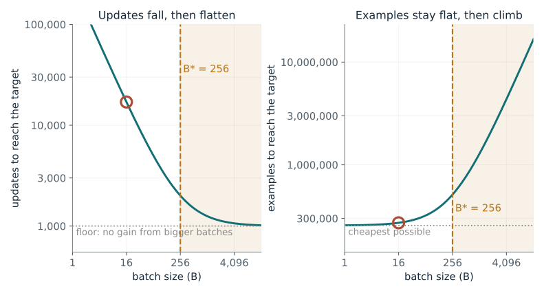
Batch size (B): 16 · Noise-to-signal ratio (B*): 256

The batch size 16 is below the critical size 256. It needs 17,000 updates and 272,000 examples. Doubling the batch to 32 would cut the updates by 47% and raise the examples by 6%.

Critical batch size (B*): 256
Updates to reach the target: 17,000
Examples to reach the target: 272,000
Examples against the cheapest possible: 1.06x

Why it matters for language models

Large language-model runs choose a batch size in tokens. Beyond the critical size, more hardware per step buys almost no speed-up but uses far more data and compute.

Show the calculation

B* = noise-to-signal ratio = 256. Updates = 1000 x (1 + B*/B) = 1000 x (1 + 256/16) = 17,000. Examples = 1000 x (B + B*) = 1000 x (16 + 256) = 272,000 (this equals B x updates); the cheapest possible is 1000 x 256 = 256,000, so this run costs 1.06x as much. At B = B*: updates are 2000 and examples are twice the minimum.

The equations and symbols

$B^*\approx\dfrac{\sigma^2}{\|\nabla F\|^2}$

$S(B)=S_{\min}\bigl(1+B^*/B\bigr)$

$E(B)=B\,S(B)=S_{\min}\,(B+B^*)$

B: batch size: examples per update
B*: critical batch size: noise-to-signal ratio sigma^2 over gradient size squared
S: updates needed to reach the target loss (floor S_min = 1000)
E: examples used in total, B times S

Where the conclusion applies

A simple noise-scale model with fixed B*, a fixed target loss, and the step size retuned for each batch. Real critical batch sizes change during training. The noise-to-signal ratio is set directly so one control covers sigma^2 and the gradient size.

Check your understanding: If B* = 1024 and you use B = 1024, how do your updates and examples compare with the floor?

Updates = 1000 x (1 + 1) = 2000, twice the floor, and examples = 1024 x 2000, twice the minimum 1000 x 1024. The knee costs a factor of two in both.

Book source: Chapter 3, Large Batches and the Limits of Scaling. Illustration C03-D08. Derived specialization. Book critical batch size B* = sigma^2/|grad F|^2 (the problem constant is set to 1). The tradeoff curves S(B) and E(B) follow the McCandlish et al. 2018 model the book cites; S_min = 1000 is a companion choice. v39 EPUB / v43 print.

Where a step size stops working

Noisy evidence and averaging

Remembering past changes

Large steps early, small steps later

Past the edge, a curved loss pulls itself back

How a stretched bowl slows descent

Learning in stages

The point where a bigger batch stops helping

Bring the idea to a question of your own