Ask for sample selection, target population, loss definition, candidate class, fitting procedure, and untouched evaluation data. Return an evaluation design and supported uncertainty calculations. Distinguish repeated-sample expectation, one observed test score, and a theorem under stated assumptions.
“My model fits every observation. What evidence supports predictions on new inputs?”
Use mathllms-ch04-generalization with the companion's AI skill package. The illustrations below also work on their own.
Bias, variance, and noise
From Chapter 4, What Complexity Actually Is
If we could retrain a model many times on fresh noisy samples, what would the repeats reveal about its mistakes?
Retraining on new noisy samples gives a cloud of fits. The cloud's average shows the systematic miss; its spread shows variance. Fresh test data adds noise on top that no fit can predict.
Predict first: With no noise at all, will a straight-line fit (degree 1) still make mistakes?
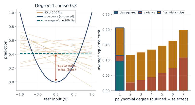
Noise level (sigma): 0.3 · Polynomial degree: 1
What happens: Yes. With zero noise every fit is the same flat line at height 5/12 (about 0.417), so variance is 0, yet the squared miss stays at 0.097. A straight line cannot bend into x squared, and more data cannot fix that.
At degree 1 the average fit misses the true curve by 0.0968 (squared) even before noise, and different training samples scatter it by 0.019. Error splits exactly into bias, variance and the noise in new data.
- Systematic miss (bias squared)
- 0.0968
- Sensitivity to the sample (variance)
- 0.019
- Noise in fresh data
- 0.09
- Total expected squared error
- 0.206
This is why a model that is too small underfits no matter how much data it sees, while one that is too flexible chases the noise in its training set; choosing model size in language models trades these two off.
Show the calculation
Averaged over 201 test inputs from -1 to 1: bias squared 0.0968 + variance 0.019 + noise 0.09 (the noise level 0.3 squared) = 0.206. The 200 seeded fits are treated as the whole population of fits, so the split is exact for them.
The equations and symbols
- f_hat
- the fitted curve (changes with each training sample)
- f_*
- the true curve; here x squared
- sigma
- noise level in the data
- degree
- highest power of x the fit may use (its flexibility)
Seed 404, 200 iid Gaussian training-noise draws conditional on nine fixed inputs in [-1, 1]. Fresh test noise has variance sigma squared. The 200 fits are treated as an equally weighted finite population, so the split is exact for them and only approximates the full expectation over all possible samples.
Check your understanding: Two retrained fits predict 1 and 3 where the true value is 1 and there is no test noise. What are bias squared, variance and total error?
Book source: Chapter 4, What Complexity Actually Is. Illustration C04-D01. Illustration. Book principle; the nine training inputs, target and noise levels are companion illustrations. v39 EPUB / v43 print.
A guarantee has a price
From Chapter 4, What Complexity Actually Is
How many examples do we need before a guarantee about a finite set of candidate models says anything useful?
To promise that every candidate's training loss is close to its true loss, you must cover the chance that some candidate got lucky. More candidates need a larger penalty, more examples a smaller one.
Predict first: What happens to the penalty if the number of examples is multiplied by four?
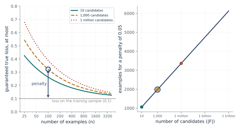
Number of examples (n): 100 · Number of candidate models: 1000
What happens: It halves, from 0.223 to 0.111. The penalty shrinks like one over the square root of n, so four times the data buys half the penalty.
With 1,000 candidates and n=100 the guarantee is training loss plus 0.223. Quadrupling n halves the penalty, while multiplying the number of candidates a thousand times adds only a little: the price of a big class is its logarithm.
- Penalty added to training loss
- 0.223
- Guaranteed true loss, at most
- 0.323
- Examples for a penalty of 0.05
- 1,981
- Confidence
- 95%
It explains why validation sets must be large enough for the number of models or settings you compared: picking the best of many candidates on one test set needs a bigger penalty.
Show the calculation
penalty = sqrt((ln 1,000 + ln 20) / (2 x 100)) = sqrt((6.91 + 3) / 200) = 0.223. Add the training loss 0.1 to get 0.323.
The equations and symbols
- n
- number of independent training examples
- |F|
- number of candidate models, fixed before seeing the data
- delta
- chance the guarantee fails (0.05 here)
- L, L_hat
- true loss and training loss (training loss 0.1 here)
A finite class chosen before seeing the data, losses in [0, 1], iid samples from the evaluation population, 0 < delta < 1. This is a uniform Hoeffding and union bound; log is the natural logarithm.
Check your understanding: Why can a network with 100 real-valued weights not use "100" as the number of candidates here?
Book source: Chapter 4, What Complexity Actually Is. Illustration C04-D02. Theorem. Book principle; the training loss 0.1, delta 0.05 and class sizes are companion illustrations. v39 EPUB / v43 print.
The interpolation peak
From Chapter 4, The Heresy of Double Descent
In a simple linear model, what exactly blows up when the number of features reaches the number of examples?
Near d = n the data matrix is almost impossible to invert, so noise in the labels is magnified into the fitted weights. Beyond d = n the fit interpolates, noise is spread thinly across many directions, and the unlearned part of the signal remains.
Predict first: If the data have no noise at all, does the curve still have a spike at d = n?
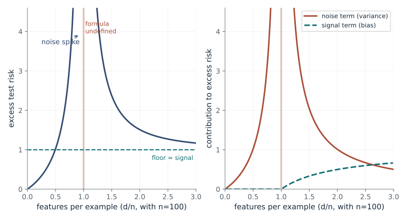
Noise variance (sigma^2): 1 · Squared signal size: 1
What happens: No. Without noise the under-parameterized side is exactly 0 and the whole spike disappears. What remains is the signal term, which climbs from 0 toward 1 as d grows past n.
At d=50 the excess risk is 1.02, at d=200 it is 1.51. The spike comes from the noise term, which blows up as d approaches n. Beyond it the noise term fades but a signal term climbs to 1.
- Excess risk at d=50
- 1.02
- Excess risk at d=200
- 1.51
- Excess risk at d=99, 100, 101
- undefined (formula needs |d - n| > 1)
- Floor for very large d
- 1
It explains why test loss can rise and then fall again as a model gets larger, the double descent seen when scaling neural networks, and why training noise matters most near the interpolation point.
Show the calculation
d=50: 1 x 50/(100-50-1) = 1.02. d=200: 1 x 100/(200-100-1) + 1 x (200-100)/200 = 1.01 + 0.5 = 1.51. Large d: the first term goes to 0 and the second to 1. Within 1 of d=n the formulas do not apply, so nothing is drawn.
The equations and symbols
- n
- number of training examples (100 here)
- d
- number of features
- sigma^2
- noise variance
- |theta*|^2
- squared size of the true coefficients (the signal)
- R
- expected test risk; excess risk is R minus sigma^2
Isotropic iid Gaussian design, correctly specified linear responses, independent homoscedastic noise, minimum-norm least squares. The signal norm is held fixed as d grows. Within 1 of d = n the formulas do not apply, and nothing is drawn there.
Check your understanding: What does the excess risk approach for very large d when the squared signal is 4?
Book source: Chapter 4, The Heresy of Double Descent. Illustration C04-D03. Illustration. Book formulas, plotted with n = 100; noise and signal levels are companion choices. v39 EPUB / v43 print.
Many perfect fits, different preferences
From Chapter 4, The Question Gradient Descent Doesn't Know It's Answering
If two models both fit every training point exactly, can they still disagree on new inputs?
The two observations constrain only one combination of the three coefficients each. Any amount of the free direction can be added without changing a training prediction, but it changes every prediction away from the training inputs.
Predict first: If we slide along the free direction, will the fit at the two observed inputs change?
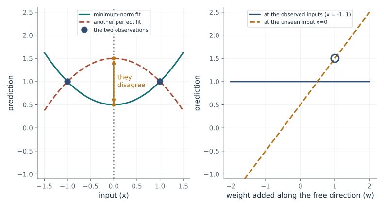
Slide along free direction (w): 1 · Unseen input (x): 0
What happens: No. At both observed inputs the prediction stays at exactly 1, yet at the unseen input x = 0 it swings from 1.5 (w = 1) to -0.5 (w = -1). The data cannot choose among these fits.
Both curves pass through the two observations exactly, yet at x=0 they predict 0.5 and 1.5. The data cannot choose between them; gradient descent from zero happens to pick the smaller, minimum-norm one.
- Misfit on the observations
- 0
- Prediction at x, minimum-norm fit
- 0.5
- Prediction at x, other fit
- 1.5
- Size of the other fit (coefficient norm)
- 1.58
Large networks have far more weights than training examples, so many exact fits exist; which one gradient descent finds is an implicit bias that shapes how the model behaves on new text.
Show the calculation
Minimum-norm coefficients (0.5, 0, 0.5). Other fit: add 1 x (1, 0, -1). At x=0: (1.5) + (-0.5) x 0^2 = 1.5. At x=-1 or 1 the extra part cancels: 1 x (1 - 1) = 0. Coefficient norm = sqrt(0.5 + 2 x (1)^2) = 1.58.
The equations and symbols
- X
- training inputs as rows (1, x, x squared) at x = -1 and x = 1
- y
- the two observed values, both 1
- theta
- coefficients of constant, linear and quadratic terms
- v
- the free direction (1, 0, -1): it changes no training prediction
- w
- how far we slide along the free direction
A consistent underdetermined linear system. Gradient descent from zero on this problem reaches the minimum-norm solution; other starting points or feature scalings can select a different one.
Check your understanding: At x = 0, what do the fits with w = -0.5 and w = 0.5 predict?
Book source: Chapter 4, The Question Gradient Descent Doesn't Know It's Answering. Illustration C04-D04. Linear specialization. Book principle; the two data points and the three features are companion illustrations. v39 EPUB / v43 print.
How well can a model class fit pure noise?
From Chapter 4, The Complexity of Noise
If we give the training points random plus-or-minus labels, how closely can the best model in the class match them?
Random signs are a pattern with no meaning. The best model in the class lines its weights up with the sum of the signed inputs. Random signs largely cancel, so that sum grows only like the square root of n while the average divides by n.
Predict first: If the number of training points grows four times, what happens to the noise-fitting score?
Training points (n): 40 · Input dimensions (d): 1
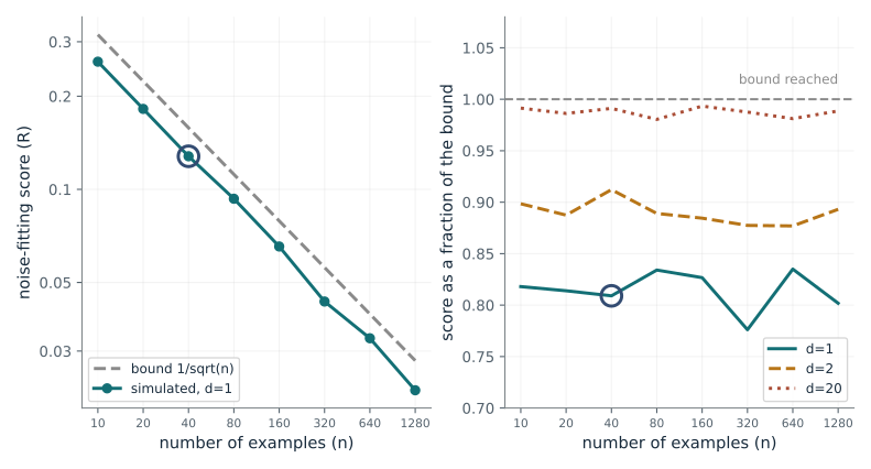
What happens: It halves, from 0.128 to 0.0654. The score follows 1/sqrt(n), parallel to the bound on the left, at about 0.8 of the bound for d = 1.
With n=40 examples the class of unit-length linear rules fits random signs to 0.128, under the bound 0.158. Both fall with slope -1/2; the dimension changes only how close the bound is, never the 1/sqrt(n) rate.
- Simulated noise-fitting score (R)
- 0.128
- Bound 1/sqrt(n)
- 0.158
- Score as a fraction of the bound
- 0.809
- Random sign patterns averaged
- 600
It shows why a model limited by weight size, not by parameter count, can generalize: the same idea underlies norm-based explanations of why heavily overparameterized networks still generalize.
Show the calculation
R = (1/n) x average over sign patterns of the length of (sigma_1 x_1 + ... + sigma_n x_n). Here n=40: 1/sqrt(40) = 0.158. Simulated average = 0.128, which is 0.809 of the bound. Four times more examples halves the bound.
The equations and symbols
- sigma_i
- a random sign, plus or minus one with equal chance
- f
- a model from the class: here w dot x with |w| at most 1
- n
- number of training points
- B_w, B_x
- size limits on weights and inputs (both 1 here)
- d
- number of input dimensions
Class {x -> w dot x : |w| at most 1} with every input of length 1. For this class the supremum equals the length of the sum of sigma_i x_i divided by n. Averages use 600 seeded sign patterns, so values carry a simulation error of a few percent. For d = 1 every input equals 1.
Check your understanding: A class has complexity 0.2 at n = 100 and follows 1/sqrt(n). What is it at n = 2,500?
Book source: Chapter 4, The Complexity of Noise. Illustration C04-D05. Theorem. Book worked example for linear functions; the inputs are random unit vectors and the sign draws are a seeded simulation. v39 EPUB / v43 print.
The spectrum behind the spike
From Chapter 4, The Heresy of Double Descent (Marchenko-Pastur law)
What happens to the eigenvalues of a random data matrix as the number of examples approaches the number of features?
Random data directions are not perfectly spread out; their strengths form an arch between two edges set by gamma. As gamma nears 1 the lower edge reaches zero, so some directions carry almost no information and fitting them requires huge weights.
Predict first: As examples per feature approaches 1, where does the lowest eigenvalue go?
Examples per feature (gamma): 0.5 · Number of examples (n): 240
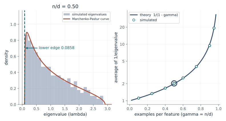
What happens: Toward zero: the allowed band starts at 0.000678 (simulated lowest 0.00106). On average inverting the eigenvalues multiplies noise by 19.5, but inverting the smallest ones multiplies it by about 1,476: the spike mechanism of the double-descent curve.
With 240 examples and 480 features the eigenvalues fill a band from 0.0858 to 2.91. As gamma nears 1 the lower edge falls to 0. Inverting them multiplies noise by 2 on average and by 11.7 at the lower edge.
- Lowest eigenvalue allowed
- 0.0858
- Highest eigenvalue allowed
- 2.91
- Lowest simulated eigenvalue
- 0.0875
- Average noise amplification 1/(1 - gamma)
- 2
It is the reason fitting a model with about as many parameters as examples is fragile: tiny eigenvalues of the data turn small label errors into large weight errors.
Show the calculation
gamma = 240/480 = 0.5; sqrt(gamma) = 0.707. Lower edge (1 - 0.707)^2 = 0.0858; upper edge (1 + 0.707)^2 = 2.91. Average of 1/lambda = 1/(1 - 0.5) = 2; at the lower edge 1/0.0858 = 11.7.
The equations and symbols
- gamma
- examples per feature, n divided by d
- lambda
- an eigenvalue of the data matrix X X-transpose
- rho
- density: the share of eigenvalues near lambda
- X
- n by d matrix of independent normal entries, variance 1/d
Large-matrix limit with iid N(0, 1/d) entries. The histogram uses one seeded n by d matrix, where d is n divided by gamma rounded to a whole number, and the theory uses the actual n/d. Finite sizes blur the edges slightly. The average of 1/lambda equals 1/(1 - gamma) in the limit, and d/(d - n - 1) exactly in expectation.
Check your understanding: For gamma = 0.25, what are the two edges of the band?
Book source: Chapter 4, The Heresy of Double Descent (Marchenko-Pastur law). Illustration C04-D06. Theorem. Book density formula; the histogram is a seeded random-matrix simulation. v39 EPUB / v43 print.
Stability from a ridge penalty
From Chapter 4, Stability as a Route to Guarantees
How strongly must a model be penalized so that swapping one training example barely changes it, and does that give a useful guarantee?
The penalty keeps weights small, so one example can move the fit only a little. That small move, summed over n examples, is what the bound turns into a promise about unseen data.
Predict first: With 100 examples and a moderate penalty (lambda = 0.5) the guarantee says nothing. Would ten times more examples make it informative?
Penalty strength (lambda): 0.5 · Number of examples (n): 100
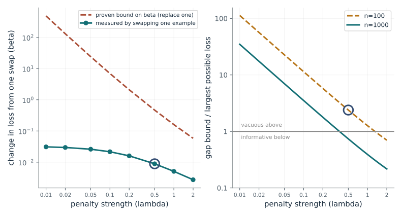
What happens: Yes. With 1,000 examples the guarantee drops from 2.39 times the largest possible loss to 0.738 times it, so it says something. A guarantee needs lambda times the square root of n to be large.
At lambda=0.5 and n=100, the worst of 6 one-example swaps moved a test loss by 0.00887, far under the proven 0.466. The resulting guarantee is 2.39 of the loss range, so it says nothing (above 1).
- Measured change from one swap (beta)
- 0.00887
- Proven bound on beta
- 0.466
- Largest possible loss (c)
- 5.83
- Gap bound as a fraction of c
- 2.39
It is the mathematical form of why weight decay and early stopping help training generalize: both limit how much any one example can move the model.
Show the calculation
c = (1/sqrt(0.5) + 1)^2 = 5.83. beta bound = 4c/(lambda n) = 4 x 5.83 / (0.5 x 100) = 0.466. Gap bound / c = 4/(lambda n) + (8/lambda + 1) x sqrt(ln 40 / (2n)) = 0.08 + 17 x 0.136 = 2.39.
The equations and symbols
- beta
- most any loss can change when one training example is swapped
- lambda
- ridge penalty strength on the squared weights
- c
- largest possible loss
- n
- number of training examples
- delta
- chance the guarantee fails (0.05 here)
Ridge regression minimizing the average squared error plus lambda times the squared weight length. Inputs have length at most 1 and labels lie in [-1, 1], so weights have length at most 1/sqrt(lambda) and the squared loss is bounded by c = (1/sqrt(lambda) + 1)^2. The measured beta is the worst of six one-example swaps over 300 test points, so it is a lower estimate of the true worst case. Five input dimensions.
Check your understanding: If lambda is halved, how does the proven bound on beta change when n stays fixed?
Book source: Chapter 4, Stability as a Route to Guarantees. Illustration C04-D07. Theorem. Book bound (Bousquet and Elisseeff). Their Theorem 22 gives 2c/(lambda n) for removing one example; the book defines stability by replacing one, which doubles it to beta = 4c/(lambda n), derived for this toy; the data are a seeded simulation. v39 EPUB / v43 print.
When the data shift: the Ben-David bound
From Chapter 4, When the Distribution Shifts
If the inputs seen after deployment differ from the training inputs, how much can the error rise, in terms we can name?
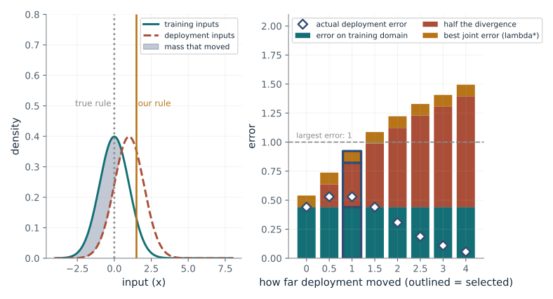
Error after deployment is at most the training error, plus how easily a model can distinguish the two domains, plus the unavoidable error of the best single model on both. The shaded region on the left is the probability mass that moved.
Predict first: As the deployment inputs move further from the training inputs, which part of the bound grows?
Deployment shift: 1 · Label noise: 0.05
What happens: The divergence term grows, from 0.383 at a shift of 1 to 0.866. The bound reaches 1.41, above 1 and so empty, while the real deployment error is only 0.109: the bound covers the worst case, not this particular classifier.
Moving the deployment inputs 1 unit adds 0.383 to the guarantee, for a bound of 0.923. The actual deployment error is 0.53 (training: 0.44). The bound stays above it, as it must.
- Error on training domain
- 0.44
- Half the divergence
- 0.383
- Best joint error (lambda*)
- 0.1
- Bound on deployment error
- 0.923
It is the reasoning behind domain adaptation and monitoring for data drift: a language model deployed on text unlike its training text can only be trusted to the degree the two are hard to tell apart.
Show the calculation
Training error = 0.05 + 0.9 x P(0 < x < 1.5) = 0.44. Half divergence = 2 x Phi(1/2) - 1 = 0.383. Best joint error = 2 x 0.05 = 0.1. Sum = 0.923. Actual deployment error = 0.53.
The equations and symbols
- L_train, L_test
- error on the training domain and on the deployment domain
- d
- divergence: how well the model class can tell the two domains apart
- lambda*
- the smallest total error any single model can reach on both domains
- shift
- how far the deployment inputs move to the right
Training inputs N(0, 1), deployment inputs N(shift, 1). The true rule is x > 0 with labels flipped with chance noise on both domains, so the labelling rule is shared. The model class is all thresholds, and our classifier is the threshold at x = 1.5. Half the divergence is then the total variation distance, 2 Phi(shift/2) - 1, and the best joint error is 2 x noise.
Check your understanding: If the deployment inputs are identical to the training inputs, which term vanishes, and what is left?
Book source: Chapter 4, When the Distribution Shifts. Illustration C04-D08. Theorem. Book bound (Ben-David et al., 2010). The Gaussian domains, true rule and classifier position are companion illustrations; every term is computed exactly. v39 EPUB / v43 print.
Bring the idea to a question of your own
Ask for sample selection, target population, loss definition, candidate class, fitting procedure, and untouched evaluation data. Return an evaluation design and supported uncertainty calculations. Distinguish repeated-sample expectation, one observed test score, and a theorem under stated assumptions.
The chapter skill can adapt the calculations to your inputs. It should identify the assumptions, explain what the result supports, and show what still needs evidence.