Chapter 6 · Convolutional and Multiscale Models

01 / 08

A filter changes what you can see

From Chapter 6, 6.2.1 Fourier Transform and Convolution Theorem

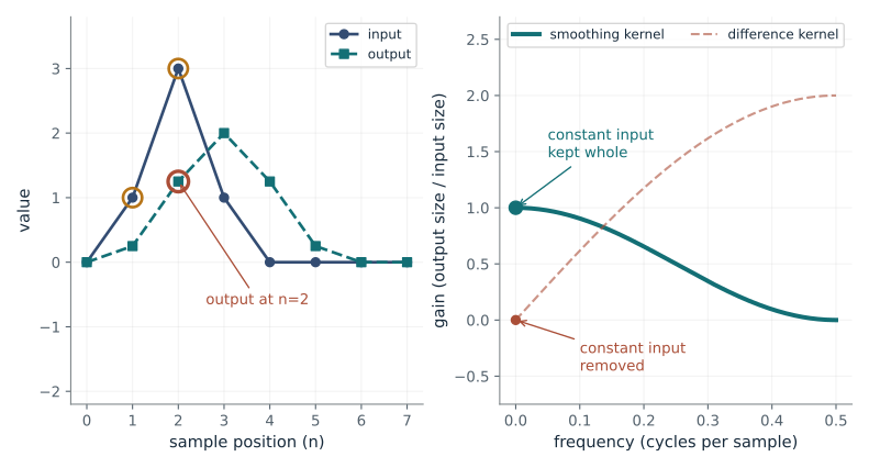
What are the actual terms in a convolution output, and what does each filter do to a flat stretch of signal?

Each output sample adds up the inputs near it, each multiplied by a kernel weight. Listing the terms shows the arithmetic, and the frequency view shows the same operation as a gain for every wave speed, where the transform of the output is the product of the transforms.

Predict first: What does each kernel do to a constant input, a perfectly flat line?

Kernel

Output sample (n): 2

07

Left: input and filtered output on eight samples with one output circled. Right: gain curves of both kernels, marked at zero frequency. — **A kernel acts differently on each frequency, and its gain at zero frequency, the sum of its weights, says what it does to a flat signal.**
Kernel: smooth · Output sample (n): 2

The smoothing kernel turns the input into the dashed output; the circled gold inputs are the ones that feed output 2. For a constant input the smoothing kernel keeps its level: its gain at zero frequency is 1.

Output at the selected sample: 1.25
Gain for a constant input: 1
Gain at the fastest wiggle: 0
Transform product versus direct sum, largest gap: 0

Why it matters for language models

Short convolutions over neighbouring tokens appear in several sequence models; whether such a kernel passes or cancels a constant level is its zero-frequency gain.

Show the calculation

Output n = sum over j of f[j] x k[(n - j) mod 8]. At n=2: 1 x 0.5 + 3 x 0.25 = 1.25. Gain at zero frequency is the sum of the kernel entries: 1. Index 0 is the kernel origin and the sum wraps around after 8 samples. The smoothing kernel (1/4, 1/2, 1/4) delays the output by one sample.

The equations and symbols

$(f*k)[n]=\sum_{j=0}^{7}f[j]\,k[(n-j)\bmod 8]$

$\operatorname{DFT}(f*k)=\operatorname{DFT}(f)\operatorname{DFT}(k)$

f: the eight input samples (0, 1, 3, 1, 0, 0, 0, 0)
k: the kernel, a short list of weights; index 0 is its origin
n: which output sample is being computed
gain: output size divided by input size for a pure wave of one frequency

Where the conclusion applies

Circular convolution on eight samples. The difference kernel is (1, -1), not a correlation. The smoothing kernel (1/4, 1/2, 1/4) is causal, so it delays the output by one sample. Frequencies are in cycles per sample, from 0 to 1/2.

Check your understanding: A kernel (1/2, 1/2) is applied to a constant signal of value 6. What comes out? What does the kernel (1, -2, 1) give?

The first gives 6 x (1/2 + 1/2) = 6, a pure smoother. The second gives 6 x (1 - 2 + 1) = 0, because its weights sum to zero. The zero-frequency gain is always the sum of the weights.

Book source: Chapter 6, 6.2.1 Fourier Transform and Convolution Theorem. Illustration C06-D01. Identity. Book convolution theorem (continuous version); this card is its eight-point cyclic analog with toy inputs. v39 EPUB / v43 print.

02 / 08

Sampling can invent a pattern

From Chapter 6, 6.2.3 Aliasing and Anti-Aliasing

Can two different tones produce exactly the same samples?

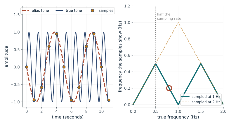
Between two samples a tone of frequency f + fs completes exactly one extra turn, so the sample values cannot show it. The samples therefore match a lower tone, and the sign of the alias tells whether that lower tone is flipped upside down.

Predict first: A tone at exactly half the sampling rate, with phase zero, is sampled. What are all the samples?

Tone frequency (Hz): 0.8

0.22

Sampling rate (Hz)

Left: a fast sine, a slower alias sine and twelve sample dots lying on both. Right: apparent frequency folds back after half the sampling rate. — **Samples keep a tone's phase only up to whole turns, so any tone above half the sampling rate shows up as a lower one.**
Tone frequency (Hz): 0.8 · Sampling rate (Hz): 1

Sampled at 1 sample per second, the 0.8 Hz tone gives exactly the samples of a -0.2 Hz tone, so the samples cannot tell them apart. Any tone above half the sampling rate folds back below it.

Alias frequency (signed, Hz): -0.2
Half the sampling rate (Hz): 0.5
Largest gap between the two sample sets: 0
Ideal low-pass filter first: removes the tone

Why it matters for language models

Audio is resampled before it reaches speech and audio models, and strided downsampling inside a network folds frequencies the same way unless the signal is smoothed first.

Show the calculation

alias = f - round(f / fs) x fs = 0.8 - 1 x 1 = -0.2 Hz. At time n/fs the two sines differ by a whole number of turns, so their samples agree (largest gap 0). A negative alias means the samples look like a sign-flipped lower tone, so the dashed curve is upside down relative to a positive sine. An ideal low-pass filter placed before sampling would remove this tone.

The equations and symbols

$\sin\!\big(2\pi (f+kf_s)\,n/f_s\big)=\sin\!\big(2\pi f\,n/f_s\big),\quad n,k\in\mathbb Z$

$f_{\mathrm{alias}}=f-\operatorname{round}(f/f_s)\,f_s$

f: true tone frequency, in hertz (cycles per second)
fs: sampling rate, in samples per second
f_alias: the signed frequency the samples appear to have
n: sample number; the sample is taken at time n / fs

Where the conclusion applies

Pure sine with phase zero, twelve samples. The low-pass step is an ideal retain-or-remove rule for this known tone, not a real finite filter. The tone is kept only if it is strictly below half the sampling rate.

Check your understanding: A sensor records 100 samples per second and a 130 Hz hum is present. What frequency will the samples show?

30 Hz: 130 - 1 x 100 = 30, which is below 50 Hz. The hum cannot be told from a real 30 Hz signal afterwards, so the signal must be filtered before it is sampled.

Book source: Chapter 6, 6.2.3 Aliasing and Anti-Aliasing. Illustration C06-D02. Identity. Book principle; the tone frequencies and sampling rates are companion toy inputs. v39 EPUB / v43 print.

03 / 08

Locate a short-lived change

From Chapter 6, 6.3.2 Continuous Wavelet Transform

Where in time does a short event sit, and how does a wavelet find it when a global frequency view cannot?

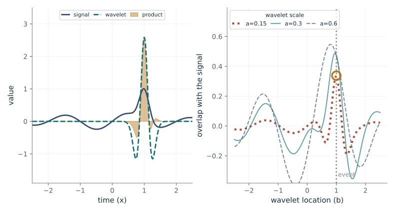
Overlap is the area under signal times wavelet. Because the wavelet has total area zero, a flat or slowly varying part of the signal cancels out, and only a feature of about the wavelet's own width, near its own location, gives a large value.

Predict first: A narrow wavelet (scale 0.15) sits on the event. Will sliding it away from the event raise or lower its overlap?

Wavelet scale (a)

Wavelet location (b): 1

-22.5

Left: a bump signal at 1 with a narrow wavelet and the shaded product. Right: overlap against location for three scales, peaking at the event. — **A wavelet overlap changes with its location, so a short event shows up as a peak at the place and scale where it sits.**
Wavelet scale (a): 0.15 · Wavelet location (b): 1

At scale a=0.15 the wavelet centered at b=1 overlaps the signal by 0.337; the gold area is that overlap. The overlap is strongest near b=1, so a wavelet can say where the short event happened.

Overlap at the chosen spot: 0.337
Strongest overlap for this scale at b: 1
Peak overlap size: 0.337
Area of the wavelet (exact): 0

Why it matters for language models

Multiscale features in vision and audio encoders that feed language models rely on this idea: use small filters for fine local detail and large ones for broad structure.

Show the calculation

Overlap = integral of f(x) x psi((x - b) / a) / sqrt(a) dx, summed on a 4001-point grid over [-4, 4]. With a=0.15 and b=1 this gives 0.337. At the wavelet center psi(0) / sqrt(a) = 1 / sqrt(0.15) = 2.58. The wavelet (1 - z^2) exp(-z^2 / 2) has total area exactly 0, so a constant signal gives zero overlap.

The equations and symbols

$Wf(a,b)=|a|^{-1/2}\int f(x)\,\overline{\psi\big((x-b)/a\big)}\,dx$

$\psi(z)=(1-z^2)\,e^{-z^2/2}$

f: the signal: a narrow bump at x = 1 plus a faint slow wave
psi: the wavelet, a small wiggle with total area zero
a: wavelet scale: how wide the wiggle is
b: wavelet location: where the wiggle is centred

Where the conclusion applies

Admissible Mexican-hat wavelet with zero area, 4001-point grid on [-4, 4]. The trapezoid sum approximates the integral and the window edge limits accuracy. Amplitudes use the 1 / sqrt(a) scale normalization.

Check your understanding: Why does a constant signal over a long window give almost zero overlap with this wavelet?

Substituting z = (x - b) / a turns the overlap into the constant times sqrt(a) times the area of the wavelet, which is zero. Cutting the window short can spoil the cancellation.

Book source: Chapter 6, 6.3.2 Continuous Wavelet Transform. Illustration C06-D03. Numerical illustration. Book wavelet definition; the Mexican-hat wavelet and the bump-plus-wave signal are companion choices. Integrals use trapezoid sums with spacing 0.002. v39 EPUB / v43 print.

04 / 08

Keep a baseline and add a correction

From Chapter 6, 6.6.2 Skip Connections and Residual Blocks; 6.6.4 ResNets as Neural ODEs

A residual block adds a correction to what it was given. Can the block still lose the information it carried?

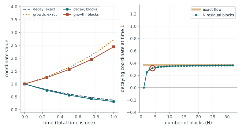
The block output is the input plus a correction. If the correction is scaled by a small step, many blocks trace out a smooth flow (the Euler method). If the correction is large relative to the identity it can cancel it.

Predict first: Strength 1 and a single block: can the block slope be zero even though the block has an identity branch?

Correction strength (alpha): 1

01.25

Blocks over time one (N)

Left: decaying and growing coordinates after N blocks against the exact flow. Right: decaying coordinate after N blocks approaching the exact value. — **An identity branch does not protect information: a correction can cancel it, and many small blocks are what approximate a smooth flow.**
Correction strength (alpha): 1 · Blocks over time one (N): 4

4 blocks of size 1/4 give 0.316 for the decaying coordinate, against 0.368 for the smooth flow. More, smaller blocks (right panel) close the gap; the identity branch alone never guarantees information survives.

Slope of one block (first coordinate): 0.75
Decaying coordinate after N blocks: 0.316
Exact flow value: 0.368
Gap between blocks and flow: 0.0515

Why it matters for language models

Transformer layers also add each layer's output to a running stream, so whether a correction can cancel or distort what it was given matters for training stability.

Show the calculation

One block multiplies the first coordinate by 1 - alpha / N = 1 - 1 / 4 = 0.75. After 4 blocks, starting from 1: (0.75)^4 = 0.316. The exact flow gives exp(-1) = 0.368. The growing coordinate uses 1 + alpha / N the same way. This is the Euler method for the pair of equations dx/dt = -alpha x and dx/dt = +alpha x.

The equations and symbols

$y=x+F_\Delta(x),\qquad J_y=I+J_{F_\Delta}$

$F_\Delta(x)=\Delta\,\operatorname{diag}(-\alpha,\alpha)\,x,\quad \Delta=1/N$

x: two coordinates, both starting at 1
alpha: correction strength: one coordinate decays, the other grows
N: number of residual blocks that share total time one
J: slope (derivative) of the block output with respect to its input

Where the conclusion applies

Linear residual map with step scaling 1 / N. Euler convergence to the flow concerns N growing at fixed strength and fixed total time, not arbitrary unscaled networks.

Check your understanding: With strength 2 and four blocks, what happens to the decaying coordinate after one block and after all four? What does the smooth flow give?

One block multiplies it by 1 - 2/4 = 0.5; four blocks give 0.5^4 = 0.0625. The smooth flow gives exp(-2) = 0.135, so four blocks are too coarse.

Book source: Chapter 6, 6.6.2 Skip Connections and Residual Blocks; 6.6.4 ResNets as Neural ODEs. Illustration C06-D04. Derived specialization. Book residual-block principle; the two-coordinate linear correction and its constants are companion toy inputs. v39 EPUB / v43 print.

05 / 08

Sharp in place or sharp in frequency

From Chapter 6, 6.2.2 Frequency Interpretation of CNN Filters

Can a window pinpoint where something happens and also exactly which frequency it has?

A narrow window changes quickly, which requires many frequencies to build it; a wide window changes slowly and needs few. Rescaling the width multiplies one spread and divides the other, so the product only depends on the shape of the window.

Predict first: Shrink the window from width 2 to width 1. Does the product of the two spreads change? Which window shape touches the limit 1 / (4 pi)?

Window shape

Window width (w): 2

0.254

Narrowing a window in position widens it in frequency by the same factor, and no window can make the product of the two spreads smaller than 1 / (4 pi).
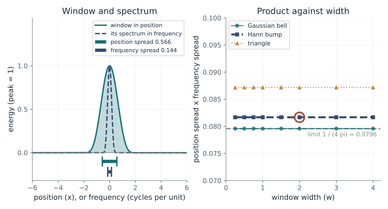
Window shape: hann · Window width (w): 2

The Hann bump of width 2 spreads 0.566 in position and 0.144 in frequency, a product of 0.0817. It sits 1.03 times above the limit. Changing the width squeezes one spread and stretches the other, leaving the product unchanged.

Spread in position: 0.566
Spread in frequency: 0.144
Product of the two spreads: 0.0817
Lowest possible product (1 / 4 pi): 0.0796

Why it matters for language models

Audio and image front ends for language models cut signals into windows; a short window locates events but blurs pitch, and a long window does the reverse.

Show the calculation

Position spread = square root of (integral of x^2 f^2 / integral of f^2) = 0.566. Frequency spread = square root of (integral of f'^2 / (4 pi^2) / integral of f^2) = 0.144. Product = 0.566 x 0.144 = 0.0817; the limit is 1 / (4 pi) = 0.0796. Halving the width halves the first factor and doubles the second. Both integrals use the exact window and its exact slope on a fine grid, so the numbers match the closed forms to the digits shown.

The equations and symbols

$\Delta x\,\Delta\xi\ \ge\ \frac{1}{4\pi}$

$\Delta x^2=\frac{\int x^2|f|^2dx}{\int|f|^2dx},\qquad \Delta\xi^2=\frac{\int \xi^2|\hat f|^2d\xi}{\int|\hat f|^2d\xi}$

Dx: spread of the window in position (standard deviation of its energy)
Dxi: spread of its spectrum in frequency, in cycles per unit
w: width setting of the window
f: the window shape: Gaussian bell, Hann bump or triangle

Where the conclusion applies

Real windows centred at zero, Fourier transform with e^(-2 pi i x xi) so frequency is in cycles per unit. A plain box window is left out because its spectrum decays too slowly for a finite frequency spread. Only the Gaussian bell attains the bound.

Check your understanding: A Gaussian window has position spread 0.5. What is its frequency spread, and could another shape do better?

Frequency spread = 1 / (4 pi x 0.5) = 0.159, since the Gaussian attains the limit. No other shape can have a smaller product, so any other shape with position spread 0.5 has a larger frequency spread.

Book source: Chapter 6, 6.2.2 Frequency Interpretation of CNN Filters. Illustration C06-D05. Inequality illustration. Book uncertainty inequality; the three window shapes and widths are companion toy inputs. Spreads are computed on a fine grid, the frequency spread through the derivative form of Parseval. v39 EPUB / v43 print.

06 / 08

Rebuild a signal from coarse to fine

From Chapter 6, 6.3.3 Multiresolution Analysis

How many numbers does a signal really need when you keep a coarse summary and add detail only where it matters?

Each step replaces neighbouring pairs by their average and their difference. The averages form a half-size summary and the differences record exactly what the summary lost, so nothing is thrown away until you choose to drop detail numbers.

Predict first: A step edge sits inside 32 samples. If you keep every level, how many of the 31 detail numbers are nonzero, and is the rebuild exact?

Signal

Detail levels kept (coarsest first): 2

05

Left: a 32-sample step with a blocky rebuild and shaded error. Right: dots by wavelet width and position, filled when kept and hollow when dropped. — **A localized feature such as an edge needs only a few wavelet numbers, one per scale, which is why coarse-to-fine summaries compress well.**
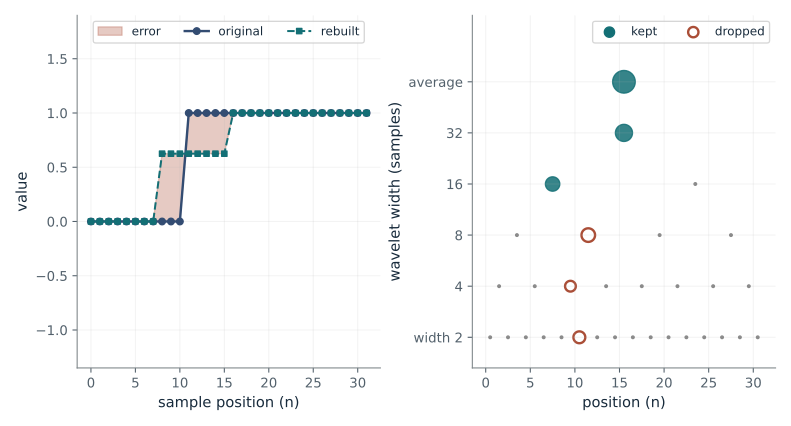
Signal: step · Detail levels kept (coarsest first): 2

Keeping the 2 coarsest detail levels (4 numbers) rebuilds the step edge with error 0.299 of its size. 5 of the 31 detail numbers are nonzero; the dots show which scales and places need them.

Numbers kept (of 32): 4
Energy kept: 91.1%
Rebuild error (share of signal size): 0.299
Nonzero detail numbers (of 31): 5

Why it matters for language models

The downsample-and-merge stages of vision and audio encoders build the same kind of pyramid, and sparse wavelet numbers are why wavelet image compression works.

Show the calculation

Each step pairs neighbours: average = (x[2n] + x[2n+1]) / sqrt(2), detail = (x[2n] - x[2n+1]) / sqrt(2). Five steps turn 32 samples into 1 average and 31 details. The squared sizes add up to the original (21). Keeping 4 numbers keeps 91.1% of that energy, so the error is sqrt(1 - 0.911) = 0.299 of the signal size.

The equations and symbols

$a_j[n]=\sum_k h[k-2n]\,a_{j+1}[k],\qquad d_j[n]=\sum_k g[k-2n]\,a_{j+1}[k]$

$h=\tfrac{1}{\sqrt2}(1,1),\quad g=\tfrac{1}{\sqrt2}(1,-1)$

a: approximation: a blurred, half-size summary of the signal
d: detail: what the blur threw away
h, g: the averaging and differencing filters of the Haar wavelet
j: level: how coarse the summary is

Where the conclusion applies

32 samples and five levels, so 1 average and 31 details. Orthonormal Haar filters, so squared sizes add up exactly. Detail levels are kept from the coarsest down. The step edge is placed at sample 11, which is not a multiple of a power of two.

Check your understanding: A constant signal of 32 equal samples is transformed. How many detail numbers are nonzero, and how few numbers rebuild it?

None: every pair has difference zero. The single average number rebuilds it, since each step just copies the average to both halves.

Book source: Chapter 6, 6.3.3 Multiresolution Analysis. Illustration C06-D06. Identity. Book fast wavelet transform with the Haar pair; the 32-sample signals are companion toy inputs. v39 EPUB / v43 print.

07 / 08

Averaging makes a shift almost invisible

From Chapter 6, 6.4.2 Mathematical Properties

If a pattern slides sideways, how much does its description change?

Raw samples of a fast wiggle change completely after a shift of a fraction of a wavelength. Taking the envelope of the wiggle and averaging it over a wide window removes the dependence on the exact position, so a shift much smaller than the window barely changes it.

Predict first: The averaging window is only 4 samples wide and the pattern shifts by 64. Is the averaged description still nearly unchanged?

Shift (samples): 16

064

Averaging scale (J, width 2^J)

Left: a wave packet, its shifted copy and their averaged envelopes. Right: change against shift for raw samples and three averaging widths. — **Averaging at width 2^J makes the description change in proportion to shift / 2^J, so it stays small for shifts well below 2^J while the raw samples change at once.**
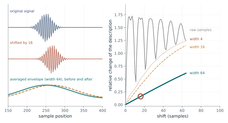
Shift (samples): 16 · Averaging scale (J, width 2^J): 6

A shift of 16 samples against an averaging width of 64: shift / 2^J = 0.25, well below the averaging width. The raw samples change by 1.66 of their size; the averaged description by 0.161, about 9.7% of that. The change grows roughly in proportion to shift / 2^J.

Change in the raw samples: 1.66
Change in the averaged description: 0.161
Shift divided by averaging width: 0.25
Averaging width (samples): 64

Why it matters for language models

Pooling layers in convolutional networks aim for the same shift tolerance; the width that buys tolerance also erases fine position detail.

Show the calculation

Relative change = norm of (description after shift - description before) / norm of description before. Raw samples: 1.66. Averaged first-order scattering with width 2^6 = 64: 0.161. The book bound says the change is at most a constant times |c| / 2^J = 16 / 64 = 0.25 (for |c| up to 2^J); the constant is not computed here.

The equations and symbols

$\|\bar S(T_cf)-\bar Sf\|\ \le\ C\,\frac{|c|}{2^{J}}\,\|f\|\quad(|c|\le 2^J)$

$\bar Sf=\big\{\,f*\phi_{2^J},\ \ |f*\psi_j|*\phi_{2^J}\,\big\}$

c: shift of the signal, in samples
J: averaging scale: the averaging window is about 2^J samples wide
phi: the smooth averaging window
psi_j: wavelet at scale j; its absolute value is the envelope of the wiggle

Where the conclusion applies

First-order scattering only, on a periodic 1024-sample signal of two wave packets. Four Gabor-style wavelets at 3 pi / 4 divided by 2^j, j = 0 to 3, and a Gaussian averaging window of standard deviation 2^J. The theorem's bound applies for shifts up to 2^J.

Check your understanding: The averaging window is 32 samples wide (J = 5). Up to what shift does the guarantee apply, and what happens to the bound if J is raised by one?

Up to about 32 samples. Raising J by one doubles the window, so the bound c / 2^J halves for the same shift, at the price of less position detail.

Book source: Chapter 6, 6.4.2 Mathematical Properties. Illustration C06-D07. Numerical illustration. Book Theorem 6.2, property 1 (the bound). The signal, the wavelets and the averaging windows are companion toy choices; the constant C is not computed, so the plot shows measured change. v39 EPUB / v43 print.

08 / 08

Convolution against attention cost

From Chapter 6, 6.10.2 Worked Example: ResNet-50 vs. ViT-B/16 Inference Compute

When an image gets bigger, does attention cost grow faster than convolution cost?

A filter does the same work at every pixel, so doubling the pixel count doubles the cost. Attention compares every patch with every other patch, so doubling the patches quadruples that comparison part. At small sizes the rest dominates, and at large sizes attention takes over.

Predict first: The transformer costs 2.1 times the convolutional network at 224 pixels. At 512 pixels, is the ratio still 2.1?

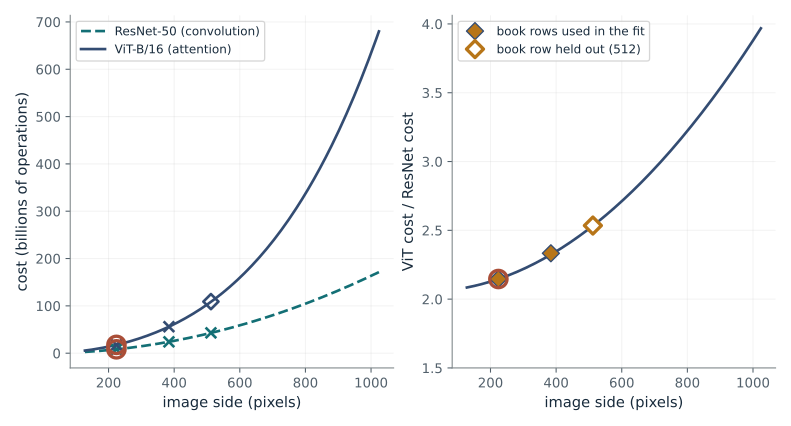
Image side (pixels): 224

2241024

Left: operations against image side for ResNet-50 and ViT-B/16 with book table points. Right: ViT over ResNet cost ratio rising with image side. — **Convolution cost grows with the number of pixels, while the attention part of a transformer grows with its square, so the cost ratio rises with resolution.**
Image side (pixels): 224

At 224 pixels the transformer costs 2.15 times the convolutional network. Convolution cost grows with the pixel count, while the attention part of the transformer grows with its square, so the ratio keeps climbing.

ResNet-50 cost: 8.2 billion
ViT-B/16 cost: 17.6 billion
ViT cost divided by ResNet cost: 2.15
Share of the ViT cost from attention: 4.27%

Why it matters for language models

Attention cost growing with the square of the number of tokens is why long inputs and high-resolution images are expensive for transformer language models.

Show the calculation

Patches N = (224 / 16)^2 = 196. ViT cost = a N + b N^2 with a = 0.08597 and b = 0.0000195 billion, fitted to the book rows 17.6 (224 px) and 56 (384 px): 16.8 + 0.751 = 17.6. ResNet cost = 8.2 x (224 / 224)^2 = 8.2. Ratio = 17.6 / 8.2 = 2.15. The book lists 109 billion for ViT at 512 px (not used in the fit); this model gives 109.

The equations and symbols

$\mathrm{FLOPs}_{\mathrm{conv}}=2K^2\,C_{\mathrm{in}}\,C_{\mathrm{out}}\,\frac{H}{s}\frac{W}{s}$

$\mathrm{FLOPs}_{\mathrm{ViT}}\approx aN+bN^2,\qquad N=(\mathrm{side}/16)^2$

K: filter size (for example 3 for a 3 by 3 filter)
Cin, Cout: number of input and output channels
N: number of 16 by 16 patches the image is cut into
a, b: constants for the part of the cost that grows like N and like N squared

Where the conclusion applies

ResNet cost scales with pixel count. ViT cost is modelled as a part linear in the patch count plus a part quadratic in it, with 16 pixel patches. This counts arithmetic only; real speed also depends on hardware, which the book notes favours the large matrix products of transformers.

Check your understanding: Attention equals the rest of the ViT cost when a N equals b N squared. At about what image side does that happen?

N = a / b = 0.0860 / 0.0000195, about 4400 patches, so the side is 16 x sqrt(4400), about 1060 pixels. Beyond that, attention is more than half of the cost.

Book source: Chapter 6, 6.10.2 Worked Example: ResNet-50 vs. ViT-B/16 Inference Compute. Illustration C06-D08. Worked example. Book table: ResNet-50 8.2 billion operations at 224 px; ViT-B/16 17.6 at 224 px, 56 at 384 px and 109 at 512 px. The two constants a and b are fitted by the companion to the 224 and 384 rows only; the 512 row is held out as a check. v39 EPUB / v43 print.

A filter changes what you can see

Sampling can invent a pattern

Locate a short-lived change

Keep a baseline and add a correction

Sharp in place or sharp in frequency

Rebuild a signal from coarse to fine

Averaging makes a shift almost invisible

Convolution against attention cost

Bring the idea to a question of your own