Chapter 7 · Recurrent and State-Space Models

01 / 08

A memory that decays

From Chapter 7, 7.9.1 Stability and BIBO Analysis

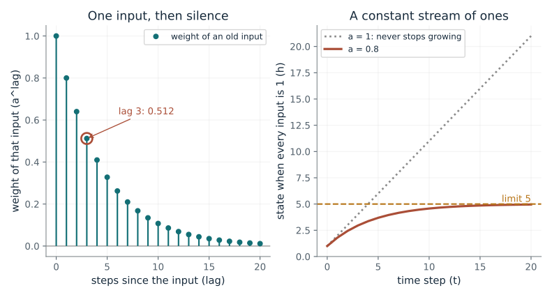
How much of an old input is still inside the state, and what happens when the inputs never stop?

Unrolling the recurrence shows that an input from L steps ago is multiplied by a, L times. A multiplier below 1 in size shrinks old inputs geometrically, so a constant stream adds up to a finite total. A negative multiplier flips the sign at every step, and a size above 1 amplifies old inputs.

Predict first: At a = 1 an isolated input is remembered perfectly. Does a bounded stream of ones then give a bounded state?

Fraction kept each step (a): 0.8

-11.2

Left: weight of an old input against lag. Right: state under a constant input of ones, with a growing reference line. — **A memory is stable only if old inputs fade: with |a| below 1 the state settles, at a = 1 it grows without bound.**
Fraction kept each step (a): 0.8

Each step multiplies old information by 0.8, so its weight dies away and a constant stream settles at 5. The state stays bounded because the weights add up to a finite total.

Weight of an input 3 steps back: 0.512
State after 3 steps of constant input: 2.95
Memory: fades
Steps for the weight to fall to 1/e: 4.48

Why it matters for language models

Recurrent networks and state-space layers repeat this one-line update over thousands of tokens, so whether their state stays bounded or explodes depends on a multiplier like a.

Show the calculation

State h_t = a h_(t-1) + u_t, starting from h = 0. An input from lag L has weight a^L, so for a = 0.8: a^3 = 0.512. For a constant input of 1: h_3 = 1 + a + a^2 + a^3 = 2.95.

The equations and symbols

$h_t=ah_{t-1}+u_t,\quad h_{-1}=0$

$\text{Weight of an input from lag }\ell=a^\ell$

a: fraction of the old state kept each step
h: the stored state (the memory)
u: the new input at each step
lag: how many steps ago the input arrived

Where the conclusion applies

Linear time-invariant scalar recurrence with zero starting state and unit input weight. Absolute stability requires |a| < 1; the time to fall to 1/e is defined only for 0 < |a| < 1.

Check your understanding: For a = -0.5 and a single input of 2 at time 0, what is the state three steps later, and does the memory fade?

2 x (-0.5)^3 = -0.25. The size shrinks by half each step while the sign flips, so it fades; it is a signed weight, not an ordinary average.

Book source: Chapter 7, 7.9.1 Stability and BIBO Analysis. Illustration C07-D01. Linear specialization. Book equation with companion toy inputs stated in the assumptions; every plotted value is recomputed. v39 EPUB / v43 print.

02 / 08

Repeated multiplication

From Chapter 7, 7.1.2 Backpropagation Through Time; 7.1.3 The Vanishing Gradient Theorem

If every step can stretch the signal by up to 1.2, must a long chain of steps blow up?

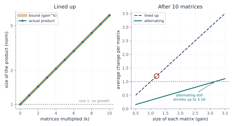
The chain rule turns the effect of an old state into a product of one Jacobian per step. A bound multiplies the sizes of the factors, which is exact only when every factor stretches the same direction. Factors that stretch different directions cancel each other, so the real product can be far smaller than the bound.

Predict first: Each matrix has size 1.2, so the bound says the product can reach 1.2^10 = 6.19. Can the real product still shrink?

Size of each matrix (gain): 1.2

0.63

How matrices are arranged

Left: size of a matrix product against length, with the bound as a wide band. Right: average change per matrix against gain, two arrangements. — **The product of sizes is only an upper bound: matrices that stretch different directions can make the true product shrink.**
Size of each matrix (gain): 1.2 · How matrices are arranged: aligned

Every matrix stretches the same direction, so the product really is as big as the bound: 6.19. Here the bound 6.19 is the truth, because it is the true size.

Size of the product after 10 matrices: 6.19
Bound from the individual sizes (gain^10): 6.19
Bound divided by the actual size: 1
Does the product grow?: yes, it grows

Why it matters for language models

Backpropagation through time multiplies one Jacobian per step, so claims that gradients must explode or vanish need the actual products, not only the size of each factor.

Show the calculation

Each matrix is 1.2 x diag(1, 0.1), size 1.2. Ten of them multiply to 1.2^10 x diag(1, 0.1^10), whose largest entry is 1.2^10 = 6.19. The bound is exact.

The equations and symbols

$\frac{\partial h_T}{\partial h_t}=J_TJ_{T-1}\cdots J_{t+1}$

$\|J_T\cdots J_{t+1}\|\leq\prod_j\|J_j\|\leq(\lambda\gamma)^{T-t}$

J: one step's Jacobian: how a change in one state moves the next
gain: the size (largest stretch) of each Jacobian
k: number of Jacobians multiplied
norm: size of a matrix: its largest stretch of any direction

Where the conclusion applies

Spectral norm, column Jacobians, prescribed diagonal matrices gain x diag(1, 0.1) and gain x diag(0.1, 1), ten matrices in each product. Later factors multiply on the left. The two arrangements are lined up (always the first matrix) or alternating.

Check your understanding: For gain 1.2, compare ten lined-up matrices with ten alternating ones. Which product is larger, and by what factor?

Lined up: 1.2^10 = 6.19. Alternating: 0.144^5 = 0.0000619. The ratio is 100000 (0.1^5 inverted), a gap that grows with every pair.

Book source: Chapter 7, 7.1.2 Backpropagation Through Time; 7.1.3 The Vanishing Gradient Theorem. Illustration C07-D02. Derived specialization. Book equation with companion toy inputs stated in the assumptions; every plotted value is recomputed. v39 EPUB / v43 print.

03 / 08

Select what to retain

From Chapter 7, 7.2.2 LSTM Architecture; 7.2.3 Gradient Highway

How does a forget gate decide how much of the old cell value survives an update?

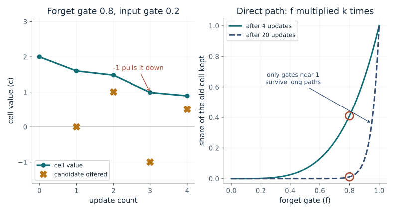
The forget and input gates separate preserving the old value from writing a new one. Prescribing them makes the recurrence transparent. The share of the starting cell that survives k updates is the forget gate multiplied k times, which collapses unless the gate is close to 1.

Predict first: With the forget gate at 1 (and the input gate at 0), will a candidate of -1 change the cell?

Forget gate (f): 0.8

01

Starting cell value (c0)

A forget gate near 1 carries a value across many updates, and the survival share is the gate multiplied along the path.
Forget gate (f): 0.8 · Starting cell value (c0): 2

With forget gate 0.8 each update keeps 80% of the old cell, so the starting value 2 is 41% present after 4 updates. The gate multiplies along the path, so only values near 1 last.

Input gate (1 - f): 0.2
Cell value after 4 updates: 0.887
Old cell kept after 4 updates (f^4): 0.41
Old cell kept after 20 updates (f^20): 0.0115

Why it matters for language models

The gated cell is the reason LSTMs can carry information across long stretches of text, because gates near 1 stop the repeated multiplication that makes plain recurrent gradients vanish.

Show the calculation

c1 = f c0 + i x 0 = 0.8 x 2 + 0.2 x 0 = 1.6. c2 = 0.8 x 1.6 + 0.2 x 1 = 1.48. Direct derivative of c4 with respect to c0 is f^4 = 0.41.

The equations and symbols

$c_t=f_tc_{t-1}+i_t\widetilde c_t$

$\text{Direct prescribed-gate derivative}=\prod_{j=1}^{T}f_j$

c: the cell value (the stored memory)
f: forget gate: share of the old cell kept
i: input gate: share of the new candidate written (here 1 - f)
candidate: the new value offered at each update: 0, 1, -1, 0.5

Where the conclusion applies

Gates are prescribed rather than learned, held constant, and the input gate is set to 1 - f. Extreme values 0 and 1 are idealized limits of sigmoid gates. The product describes the direct path only, not every dependency of a trained LSTM.

Check your understanding: With f = 0.9, how much of the starting cell value is still there after 10 updates along the direct path?

0.9^10 = 0.349, about 35%. A gate of 0.9 sounds high, but it still loses two thirds of the value in 10 steps.

Book source: Chapter 7, 7.2.2 LSTM Architecture; 7.2.3 Gradient Highway. Illustration C07-D03. Prescribed-gate specialization. Book equation with companion toy inputs stated in the assumptions; every plotted value is recomputed. v39 EPUB / v43 print.

04 / 08

The same memory, two descriptions

From Chapter 7, 7.3.4 Dual Computation Modes

Does running the memory step by step give the same output as summing weighted past inputs, and when does it not?

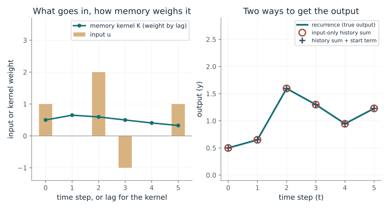
Unrolling a fixed linear update gives a kernel: the weight of an input depends only on how long ago it arrived. Summing kernel times inputs reproduces the step-by-step output exactly. The memory the system starts with also fades through the same kernel, so it must be added as its own term.

Predict first: If the memory starts non-empty, can the same input-only history sum still match the recurrence?

First state multiplier (a): 0.8

0.30.95

Starting memory

Left: input bars and the memory kernel by lag. Right: output from the recurrence, the input-only history sum and the corrected sum. — **Step-by-step and history-sum computation agree exactly when the start is empty; a nonzero start adds one extra fading term.**
First state multiplier (a): 0.8 · Starting memory: zero

Both descriptions give the same output at every step: the circles sit exactly on the line, and the plus marks sit on the circles because the start term is zero.

Kernel weight at lag 0 (K0): 0.5
Kernel weight at lag 1 (K1): 0.65
Output at step 2 (recurrence): 1.6
Largest gap, recurrence vs history sum: 0

Why it matters for language models

State-space language models train in the fast history-sum (convolution) form and generate in the step-by-step form, so the two must agree, including how the starting memory is handled.

Show the calculation

A = diag(0.8, 0.3), B = (1, 0.5), C = (1, -1), so K0 = C B = 1 - 0.5 = 0.5 and K1 = 0.8 - 0.15 = 0.65. History sum at t = 2: K2 u0 + K1 u1 + K0 u2 = 0.595 + 0 + 1 = 1.595. Start term at t = 2: 0. Recurrence: 1.595.

The equations and symbols

$h_t=\bar A h_{t-1}+\bar B u_t,\quad y_t=Ch_t$

$y_t=\sum_{s=0}^{t}C\bar A^{t-s}\bar B u_s+C\bar A^{t+1}h_{-1}$

A-bar: how the state carries over one step: diag(a, 0.3)
B-bar, C: write weights (1, 0.5) and read weights (1, -1)
K: the kernel: weight of an input by its lag
h(-1): the memory before the first input

Where the conclusion applies

Constant matrices, no direct feedthrough, input u = (1, 0, 2, -1, 0, 1) indexed from t = 0. The nonzero start is h(-1) = (1, 0.5). Recurrence and history sum share the same indexing.

Check your understanding: For a nonzero starting state, what term must be added to the history sum at time t?

C A-bar^(t+1) h(-1), the fading echo of the starting memory. The exponent is t + 1 because the first update already applies A-bar once.

Book source: Chapter 7, 7.3.4 Dual Computation Modes. Illustration C07-D04. Identity. Book equation with companion toy inputs stated in the assumptions; every plotted value is recomputed. v39 EPUB / v43 print.

05 / 08

A polynomial memory of everything so far

From Chapter 7, 7.15.1 HiPPO on a Sine Wave; 7.4.2 HiPPO-LegS

Can a handful of numbers remember a whole stretch of a signal, and how long a stretch before they fail?

The memory stores the Legendre coefficients of everything seen so far, which is the best polynomial fit to the whole window. For one smooth period the coefficients shrink very fast, so a few are enough. A polynomial of degree m-1 can cross zero at most m-1 times, so a window with more crossings than that cannot be followed, whatever the coefficients.

Predict first: Eight numbers rebuild one period of the sine to better than 0.001. Does the same eight-number memory still work when the window grows to ten periods?

State size (m): 8

216

Window length (periods)

Left: a sine and its polynomial reconstruction with the error shaded. Right: correct decimal places against state size for three window lengths. — **A fixed-size polynomial memory is accurate while the window is smooth enough for its degree, and fails once the signal wiggles more than the polynomial can.**
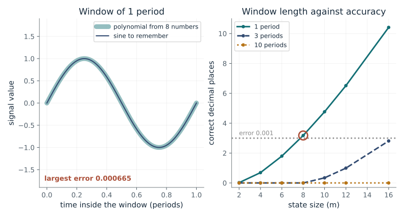
State size (m): 8 · Window length (periods): 1

8 Legendre numbers rebuild the sine to within 0.000665. The polynomial has room for the 1 zero crossing, and the coefficients shrink fast, so a handful of numbers hold the whole window.

Largest error over the window: 0.000665
Correct decimal places: 3.2
Zero crossings the sine has in the window: 1
Most a polynomial of degree m-1 can have: 7

Why it matters for language models

HiPPO is how some state-space layers keep a fixed-size summary of a long history, and this limit shows why the state size must grow with how detailed the remembered signal is.

Show the calculation

The state is the best polynomial of degree 7. Window: 1 period, so sin(2 pi s) has 1 interior zero crossing; a polynomial of degree 7 has at most 7. Largest error 0.000665. For contrast, an RNN with |lambda| = 0.99 keeps 0.99^10 = 0.904 of an input from 10 steps ago and 0.99^100 = 0.366 from 100.

The equations and symbols

$c_n(t)=\frac{2n+1}{t}\int_0^t u(s)\,P_n\!\left(\tfrac{2s}{t}-1\right)ds$

$u(s)\approx\sum_{n=0}^{m-1}c_n(t)\,P_n\!\left(\tfrac{2s}{t}-1\right)$

m: state size: the number of Legendre coefficients kept
c_n: the n-th coefficient, one number of the memory
P_n: Legendre polynomial of degree n
window: the stretch [0, t] of time being remembered, measured in sine periods

Where the conclusion applies

Signal sin(2 pi s) on a window of 1, 3 or 10 periods. The memory is the best degree m-1 polynomial in the average-squared-error sense, with standard (unnormalized) Legendre polynomials; the fitted curve is the same as the book's normalization. Error is the largest gap over the window.

Check your understanding: A signal crosses zero 7 times inside the window. What is the smallest state size m that could possibly follow it?

A degree m-1 polynomial has at most m-1 crossings, so m-1 must be at least 7 and m at least 8. That is necessary only; the shape must also fit.

Book source: Chapter 7, 7.15.1 HiPPO on a Sine Wave; 7.4.2 HiPPO-LegS. Illustration C07-D05. Worked example. Book worked example (u = sin(2 pi s), m = 8). The coefficients are the exact least-squares projection computed by quadrature; the HiPPO differential equation is not simulated. v39 EPUB / v43 print.

06 / 08

Turning a continuous memory into steps

From Chapter 7, 7.3.3 Discretization

When a continuous memory is sampled in steps, why is the exact "zero-order hold" rule safer than the naive Euler rule?

The exact solution over one step multiplies the state by e raised to minus rate times step, always between 0 and 1. Euler replaces that with the first two terms, 1 minus rate times step, which goes negative and then grows past size 1 for large steps. Both agree for tiny steps.

Predict first: Euler multiplies the state by 1 - z each step. What happens when the step is larger than 2 divided by the rate?

Step size (Delta): 1.5

0.13

Decay rate

Left: exact state curve with ZOH and Euler steps. Right: one-step multiplier size of both rules against step times rate. — **Zero-order hold keeps a decaying memory decaying at any step size; Euler becomes unstable once step times rate passes 2.**
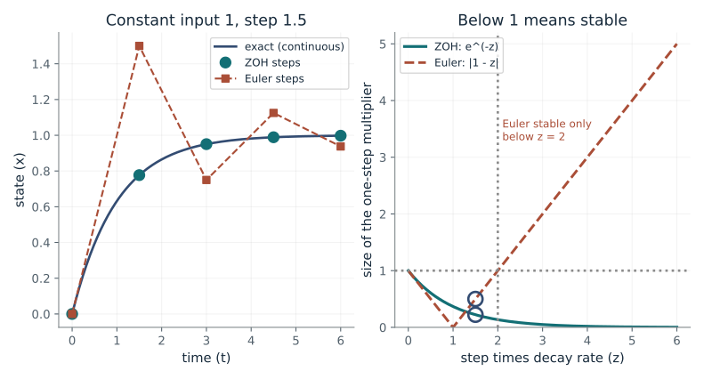
Step size (Delta): 1.5 · Decay rate: 1

The ZOH steps land exactly on the true curve for any step size. Euler multiplies by -0.5 each step: stable here, but off by up to 0.723.

ZOH multiplier e^(-z): 0.223
Euler multiplier 1 - z: -0.5
Euler worst error at the steps: 0.723
Euler verdict: stable

Why it matters for language models

State-space language models learn the step size Delta, and the exponential form guarantees a stable decaying memory however large Delta becomes.

Show the calculation

Model x' = -1 x + u. z = 1 x 1.5 = 1.5. ZOH: A-bar = e^(-z) = 0.223, B-bar = (1 - e^(-z)) / 1 = 0.777. Euler: A-bar = 1 - z = -0.5, B-bar = 1.5. Steady state is 1/1 = 1 for both when stable.

The equations and symbols

$\bar A=e^{A\Delta},\quad \bar B=A^{-1}(e^{A\Delta}-I)B$

$\bar A_{\text{Euler}}=1+A\Delta,\quad \bar B_{\text{Euler}}=\Delta B$

A: continuous decay: here A = -rate
Delta: step size (time between samples)
z: step size times decay rate, the one number that sets stability
A-bar, B-bar: per-step multiplier and input weight

Where the conclusion applies

Scalar model x' = -rate x + u with a constant input of 1 and starting state 0, observed until time 6. Zero-order hold is exact when the input is constant between samples, which holds here. Rates 1 and 2.

Check your understanding: With decay rate 4, what is the largest step Euler can use and stay stable, and does ZOH have such a limit?

Euler needs |1 - 4 Delta| below 1, so Delta below 0.5. ZOH multiplies by e^(-4 Delta), always between 0 and 1, so it has no limit.

Book source: Chapter 7, 7.3.3 Discretization. Illustration C07-D06. Derived specialization. Book equation with companion toy inputs stated in the assumptions; every plotted value is recomputed. v39 EPUB / v43 print.

07 / 08

Letting each token pick its own timescale

From Chapter 7, 7.5.2 Selective SSMs

Can a memory write one important token strongly and still ignore the filler around it?

The step size Delta decides two things at once. The old state is kept by a factor e^(-Delta), so small Delta keeps it. The new token is written with strength 1 - e^(-Delta), so small Delta also skips the token. Making Delta depend on the token lets the model skip filler and write key tokens.

Predict first: What timescale should the key token get, and what should the fillers get, if the model wants the key to survive?

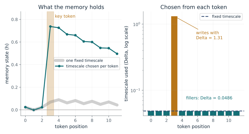
Key-token boost (w): 4

010

Left: memory state over 12 tokens, selective against fixed timescale. Right: bars of the timescale used for each token, tall at the key token. — **Choosing the timescale per token lets the memory write the key hard and then skim over filler, which no fixed timescale can do.**
Key-token boost (w): 4

The key token gets timescale 1.31 and is written with strength 0.731; fillers get 0.0486 and each writes only a small step. The key contributes 0.496 to the final state, against 0.0322 with one fixed timescale.

Timescale at the key token: 1.31
Timescale at filler tokens: 0.0486
Key token left in the final state: 0.496
Key weight / filler weight: 2.86

Why it matters for language models

This is the selection mechanism in Mamba-style models: tokens decide how much of the state to overwrite, which is how a fixed-size state can hold what matters in a long prompt.

Show the calculation

Delta = softplus(-3 + w x flag). Filler: softplus(-3) = 0.04859, so e^(-Delta) = 0.9526 (keeps most) and the write is 1 - e^(-Delta) = 0.04743. Key with w = 4: Delta = 1.313, write = 0.7311. Eight fillers follow the key, each keeping 0.9526, so the key keeps 0.731 x 0.678 = 0.496.

The equations and symbols

$\Delta_t=\operatorname{softplus}(s_\Delta(x_t))$

$\bar A_t=e^{A\Delta_t},\quad \bar B_t=A^{-1}(e^{A\Delta_t}-1)B$

Delta_t: timescale chosen from token t
A: fixed decay, here -1
w: how strongly the key token raises its own timescale
e^(-Delta): share of the old state kept at this step

Where the conclusion applies

Scalar state, A = -1, B = 1, 12 tokens: one key token with value 1 at position 3 and alternating filler values +0.5, -0.5. The timescale is softplus(-3 + w x flag), where flag marks the key token. w = 0 is the fixed-timescale baseline.

Check your understanding: If the model sets a filler token's timescale to nearly zero, what happens to the state at that step?

e^(-Delta) is near 1, so the old state is kept almost unchanged, and the write 1 - e^(-Delta) is near 0, so the filler is skipped.

Book source: Chapter 7, 7.5.2 Selective SSMs. Illustration C07-D07. Derived specialization. Book equation; the token stream, the bias -3 and the scalar state are companion toy choices. v39 EPUB / v43 print.

08 / 08

A complex memory inside the unit circle

From Chapter 7, 7.11.2 LRU: Linear Recurrent Unit; 7.11.3 Input Normalization for Linear Recurrences

What do the size and the angle of a complex multiplier do to a memory, and why does the angle matter for constant inputs?

Writing the multiplier as r times a rotation separates two jobs: r makes the memory fade, 1/nu steps to fall to 1/e, and the angle makes it swing like a damped pendulum. The steady response to a constant input is 1 over the distance from lambda to 1. That distance is small only when lambda is real and close to 1.

Predict first: A real multiplier 0.99 turns a constant input of 1 into a state of 100. If the same multiplier size also rotates by one tenth of a turn per step, does the state stay near 100?

Decay strength (nu): 0.01

0.0010.3

Turns per step

Left: the memory spiralling inside the unit circle. Right: steady response to a constant input against decay, four rotation speeds. — **The size r sets how long a memory lasts, and the angle sets how it oscillates; a near-1 real multiplier amplifies constant inputs but a rotating one does not.**
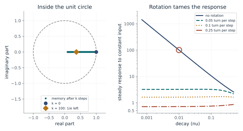
Decay strength (nu): 0.01 · Turns per step: 0

A real eigenvalue 0.99 just fades along the axis, and a constant input piles up to 101 times its size, the 1/(1-r) growth. LRU normalization keeps the variance of random inputs bounded, but for a constant input it only slows this growth.

Memory left after one step (r = e^-nu): 0.99
Steps for memory to fall to 1/e: 100
Steps per full turn: undefined (no rotation)
Steady response to constant input: 101

Why it matters for language models

The Linear Recurrent Unit keeps every entry inside the unit circle so training is stable, and its input normalization keeps the variance of random inputs bounded even for near-1 entries; for a steady input it only slows the growth, it does not stop it.

Show the calculation

lambda = r e^(i theta), r = e^(-0.01) = 0.99, theta = 2 pi x 0 = 0 rad. Memory length 1/nu = 100 steps. Response to a constant input of 1 is 1/|1 - lambda|, where |1 - lambda|^2 = 1 - 2 r cos(theta) + r^2 = 9.901 x 10^-5, so it equals 101.

The equations and symbols

$\bar\lambda=re^{i\theta},\quad r=e^{-\nu},\ \theta\in[0,\pi]$

$h_k\to\frac{\bar b\,u}{1-\bar\lambda}\quad(k\to\infty)$

r: how much memory survives one step (below 1)
nu: decay strength: r = e^(-nu), memory length 1/nu steps
theta: angle turned per step; one full turn is 2 pi
lambda: the complex multiplier r e^(i theta)

Where the conclusion applies

One diagonal entry, input weight 1, constant input 1. Decay values 0.001 to 0.3 and rotations of 0, 0.05, 0.1 and 0.25 turns per step. The steady response is the limiting value and exists because r < 1.

Check your understanding: An entry has decay nu = 0.01 and one turn every 10 steps. Is its constant-input response near 100?

No. |1 - lambda| is about 0.62, so the response is about 1.6. Only a positive real entry with the same size would give 100.

Book source: Chapter 7, 7.11.2 LRU: Linear Recurrent Unit; 7.11.3 Input Normalization for Linear Recurrences. Illustration C07-D08. Derived specialization. Book equation with companion toy inputs stated in the assumptions; every plotted value is recomputed. v39 EPUB / v43 print.

A memory that decays

Repeated multiplication

Select what to retain

The same memory, two descriptions

A polynomial memory of everything so far

Turning a continuous memory into steps

Letting each token pick its own timescale

A complex memory inside the unit circle

Bring the idea to a question of your own