Chapter 8 · Attention and Transformers

01 / 08

Which values reach the current token?

From Chapter 8, 8.1.1 The Attention Operation; 8.1.4 Causal (Masked) Attention; 8.3 The Transformer Block

How do three query-key comparisons become a weighted output, and what does a causal mask remove?

A dot product measures how a query aligns with each key, and division by the square root of width sets the score scale. Row softmax turns those scores into a distribution, then the output averages the value vectors using that distribution. A mask changes which keys can contribute before the average is formed.

Predict first: Select token 1 with the causal mask on. Which value vector must its output equal?

Inspect query token

Allowed context

Two colored 3 by 3 grids, scores and softmax weights, with the selected query row boxed and masked future cells hatched. — **A mask removes keys before softmax, so a blocked token receives exactly zero weight and the remaining weights still add to 1.**
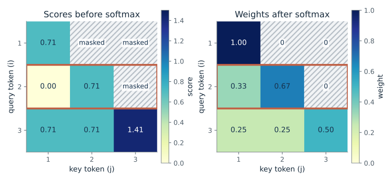
Inspect query token: 2 · Allowed context: causal

Token 2 mixes the three value vectors with weights (0.33, 0.67, 0.00), giving the output (0.33, 1.34). Hatched cells are masked, so later tokens get exactly 0. These weights describe a calculation, not proof that any input is true.

Weights on tokens 1, 2, 3: 0.330, 0.670, 0.000
Tokens this query may use: 1, 2
Row of weights adds to: 1.000
Weighted output: (0.330, 1.340)

Why it matters for language models

A language model that writes one token at a time must not read the tokens it has yet to write; the causal mask is how training enforces that, and it is why the earliest tokens can only attend to a short prefix.

Show the calculation

First output coordinate: 0.330 x 1 + 0.670 x 0 + 0.000 x 2 = 0.330. Second: 0.330 x 0 + 0.670 x 2 + 0.000 x 1 = 1.340. Scores are query-key dot products divided by sqrt(2) = 1.414, then each row is passed through softmax over its allowed keys.

The equations and symbols

$S=\frac{QK^\top}{\sqrt{d}},\qquad A_{ij}=\frac{\exp(S_{ij}+M_{ij})}{\sum_\ell\exp(S_{i\ell}+M_{i\ell})},\qquad Z=AV$

$M_{ij}=\begin{cases}0&j\leq i\\-\infty&j>i\end{cases}\quad\text{for causal attention}$

Q, K, V: query, key and value vectors, one row per token
d: vector width (here 2)
S: scores: query-key dot products divided by sqrt(d)
M: mask: 0 where allowed, minus infinity where blocked
A: weights: each row is positive and adds to 1
Z: output: each row is a weighted average of the value rows

Where the conclusion applies

Softmax is applied across each query's allowed keys. Causal masking allows the diagonal j = i, so no row is empty; next-token training uses shifted targets. A fully masked row would have undefined normalization and is rejected. Positive weights sum to one.

Check your understanding: For causal query 1, what are the weights and output even though its unmasked dot product with key 3 is positive?

The weights are (1, 0, 0), so the output is V1 = (1, 0). Future key 3 is masked before normalization and contributes zero.

Book source: Chapter 8, 8.1.1 The Attention Operation; 8.1.4 Causal (Masked) Attention; 8.3 The Transformer Block. Illustration C08-D01. Identity. Book attention equation, expressed with tokens as rows (the book also presents an equivalent column convention). The three vectors are illustrative; this is one attention head, without projection, residual, normalization, or feed-forward stages. v39 EPUB / v43 print.

02 / 08

Change variety without confusing it with accuracy

From Chapter 8, 8.10.1 Temperature Scaling; 8.10.2 Truncation: Top-k and Nucleus Sampling

What happens between a model's fixed logits and a sampled next token?

Temperature rescales differences between logits before softmax; a smaller positive T sharpens preferences that already exist. Nucleus sampling then removes the smallest-probability tail and rescales the retained mass to one. A finite draw count fluctuates around its expectation even when the distribution is fixed.

Predict first: Lower T from 1 to 0.5 with the cut at 0.9. Does token A gain probability, and does the kept set get smaller?

Temperature (T): 1

0.254

Nucleus threshold (alpha)

Left: paired bars for four tokens before and after the nucleus cut. Right: four probability curves against temperature with a marker. — **Lower temperature piles probability onto the leading token, and the nucleus cut then keeps fewer tokens; neither step tests whether a token is correct.**
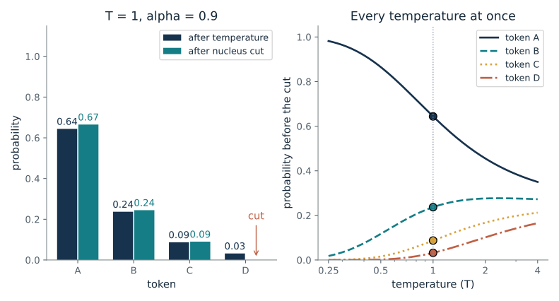
Temperature (T): 1 · Nucleus threshold (alpha): 0.9

At T = 1 the cut keeps A, B, C with total mass 0.968, then rescales them to sum to 1. Lowering T further would move more probability onto A and could shrink the kept set. None of this checks whether a token is true.

Tokens kept by the cut: A, B, C
Probability mass kept: 0.968
Final probability of A: 0.665
A in 200 repeatable draws: 150 (expected 133)

Why it matters for language models

Sampling settings in a chat assistant are exactly these two knobs. They change how much wording varies between runs, not how likely an answer is to be factually right.

Show the calculation

A starts at 0.644. Final probability = 0.644 / 0.968 = 0.665. Expected count in 200 draws = 133.0; the fixed run (seed 20260929) drew A 150 times.

The equations and symbols

$p_T(i)=\frac{\exp(z_i/T)}{\sum_j\exp(z_j/T)},\qquad T>0$

$S_\alpha=\text{smallest probability-sorted prefix with }\sum_{i\in S_\alpha}p_T(i)\geq\alpha,\qquad \widetilde p(i)=\frac{p_T(i)\mathbf{1}_{i\in S_\alpha}}{\sum_{j\in S_\alpha}p_T(j)}$

z: fixed logits (2, 1, 0, -1) for tokens A to D
T: temperature, always positive; small T sharpens
alpha: nucleus threshold: keep tokens until their mass reaches alpha
p-tilde: final probabilities after the cut and rescaling

Where the conclusion applies

T stays strictly positive. Tokens are sorted by descending probability with a stable original-order tie rule; the token crossing alpha is retained. Alpha = 1 keeps the entire support. The logits have a unique maximum; tied maxima would approach a uniform distribution over the tied maximizers as T tends to zero.

Check your understanding: If the retained probabilities originally sum to 0.8 and one retained token has probability 0.4, what is its final probability? Does that number certify truth?

Its final probability is 0.4/0.8 = 0.5. This is its sampling probability among the retained tokens, with no factual verification implied.

Book source: Chapter 8, 8.10.1 Temperature Scaling; 8.10.2 Truncation: Top-k and Nucleus Sampling. Illustration C08-D02. Identity and simulation. Book probability transformations; fixed logits are illustrative. The 200 draws use NumPy default_rng with seed 20260929 and are recomputed for each selected distribution. v39 EPUB / v43 print.

03 / 08

Keep the gap while moving both positions

From Chapter 8, 8.2.5 Rotary Positional Encoding (RoPE); 8.7.3 Worked Example: RoPE Attention Scores

Why can rotating a query and a key encode their relative separation?

Rotating both vectors introduces two absolute angles, but their dot product depends on the angle difference. Orthogonality cancels the common rotation, leaving only the relative gap for fixed content. Different coordinate pairs rotate at different rates, so a single gap affects several positional scales at once.

Predict first: Both positions are already shifted by 990 tokens, and the gap is 100. Widen the gap to 300 tokens. Does the dot product change, and is it the shift or the gap that moves it?

Gap between positions (tokens): 100

0400

Shift both positions

Left: query and key arrows on a circle with the gap arc. Right: dot product against gap with the current and shift-zero scores marked. — **Rotating the query and the key by position makes their dot product depend only on the gap between them.**
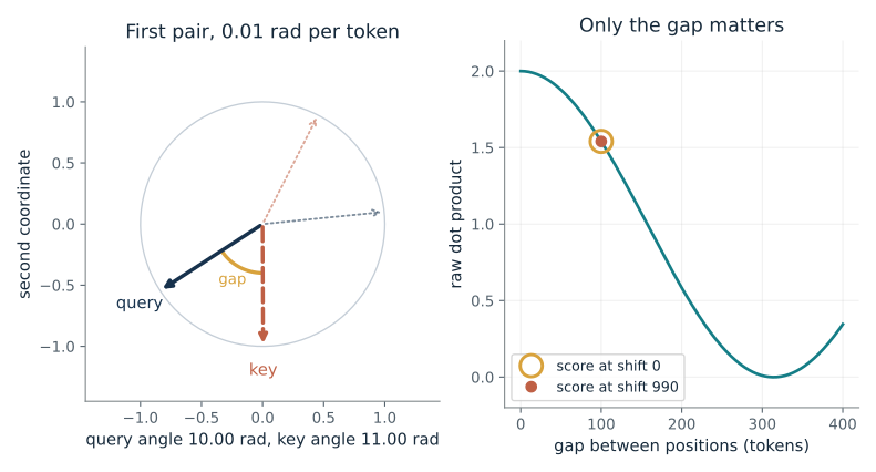
Gap between positions (tokens): 100 · Shift both positions: 990

The query sits at position 1000 and the key at 1100. Moving both by 990 turns each arrow by the same extra angle, so the angle between them, and the dot product 1.54, stay put. The curve reads the same value at every shift.

Positions (query, key): 1000, 1100
Dot product, both rotated: 1.54
Dot product, gap rotation only: 1.54
Scaled attention score (raw / 2): 0.77

Why it matters for language models

Rotary position lets attention know how far apart two tokens are without storing absolute positions, which is how many current language models encode word order.

Show the calculation

Raw score = cos(0.01 x 100) + cos(0.0001 x 100) = 0.54 + 1 = 1.54. Computing it from the two absolute rotations gives the same number (difference 0). Dividing by sqrt(4) = 2 gives the scaled score 0.77.

The equations and symbols

$R_t=\operatorname{diag}(R(t\theta_1),R(t\theta_2)),\quad R(a)=\begin{pmatrix}\cos a&-\sin a\\\sin a&\cos a\end{pmatrix}$

$(R_tq)^\top(R_sk)=q^\top R_t^\top R_sk=q^\top R_{s-t}k$

q, k: fixed content vectors, both (1, 0, 1, 0)
t, s: positions of the query and the key (tokens)
R_t: rotation by an angle proportional to position t
theta: turn per token: 0.01 and 0.0001 rad for the two pairs
s - t: the gap between the two positions

Where the conclusion applies

Query and key content vectors and frequencies remain fixed while positions move. Each block is an orthogonal rotation, with R_t transpose R_s = R_(s-t). Real model hidden states may change when text moves or is inserted. No claim about successful long-context extrapolation follows from this identity alone.

Check your understanding: What is the raw score for gap 2, and what is the corresponding scaled score at width 4?

The raw score is cos(0.02) + cos(0.0002), about 1.9997999867. Dividing by sqrt(4) gives about 0.9998999933.

Book source: Chapter 8, 8.2.5 Rotary Positional Encoding (RoPE); 8.7.3 Worked Example: RoPE Attention Scores. Illustration C08-D03. Identity. Book worked example: q = k = (1,0,1,0), t = 10, s = 12, frequencies (0.01, 0.0001). Other gaps and common shifts are extensions of that exact calculation. v39 EPUB / v43 print.

04 / 08

Count context cost in the right units

From Chapter 8, 8.5 Efficient Attention; 8.5.1 The Quadratic Bottleneck; 8.11.3 Cache Size: Linear in Sequence Length, Not Constant

Which costs grow quadratically with context, and which grow linearly?

Each query compares with each key, producing n squared scores independently of head width. Increasing width makes each comparison and weighted sum more expensive and makes cached vectors larger. The cache comparison includes every ordinary KV head rather than comparing a shared latent against just one head. Compressing per-token cache width reduces a constant factor; the number of cached tokens still grows with context.

Predict first: Double the context length from 256 to 512 while holding width fixed. By what factor do the score entries and each cache grow?

Context length (n tokens): 256

162048

Head width (d)

Left: n and n squared lines on one log axis with the gap at the chosen n marked. Right: ordinary and compressed cache sizes against n. — **Pairwise scores grow as n squared but stored keys and values grow as n, so long contexts cost most in the pairwise parts.**
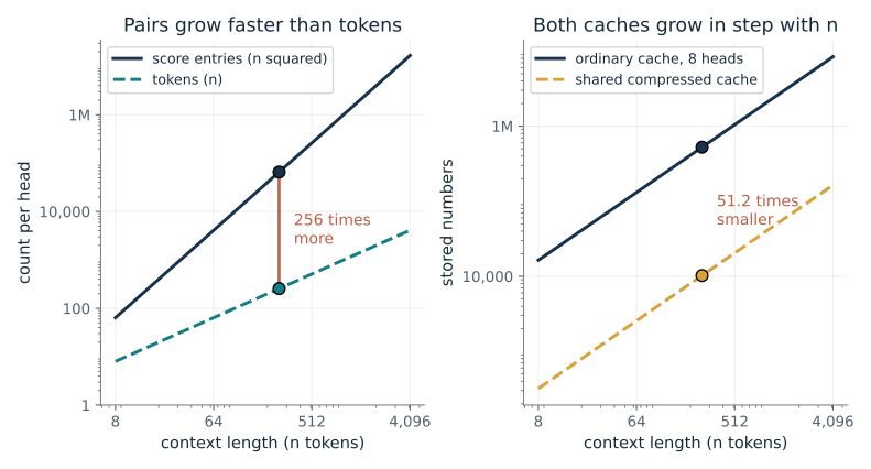
Context length (n tokens): 256 · Head width (d): 128

At n = 256 tokens one head forms 65,536 scores, 256 times the token count. Doubling n quadruples the scores but only doubles each cache. These are counts, not measured run times.

Score entries per head: 65,536
Attention arithmetic per head: 16,777,216 multiply-adds
Ordinary cache (8 heads): 524,288 numbers
Shared compressed cache: 10,240 numbers (51.2 times smaller)

Why it matters for language models

This is why pasting a much longer document is not free: the attention work per layer grows with the square of the length, and the cache that must be kept in memory grows with the length itself.

Show the calculation

Scores: 256 x 256 = 65,536. Arithmetic: 2 x 256^2 x 128 = 16,777,216. Ordinary cache: 2 x 256 x 8 x 128 = 524,288. Compressed: 256 x (32 + 8) = 10,240.

The equations and symbols

$\#\text{scores}=n^2,\qquad \text{dense QK and AV arithmetic}\approx 2n^2d\ \text{MACs}$

$\text{ordinary full-layer KV values}=2nn_hd,\qquad \text{compressed cache values}=n(d_c+d_R)$

n: context length in tokens
d: width of one attention head
n_h: key-value heads in the ordinary cache (8 here, illustrative)
d_c, d_R: compressed width d/4 and rotary width 8 (illustrative)
MAC: one multiply-add operation

Where the conclusion applies

Dense full-sequence attention in one layer. Score and arithmetic counts describe one head; the cache panel compares all eight ordinary KV heads with one layer-shared compressed cache. Key and value head widths equal d. Arithmetic counts QK and AV only; it excludes projections, softmax, feed-forward layers, and runtime overhead. Score storage assumes materializing all n squared scores; tiled exact attention can avoid that storage without removing quadratic dense arithmetic. Both cache schemes grow linearly in n.

Check your understanding: At n = 16, d = 32 and eight KV heads, how many per-head score entries and full-layer ordinary KV values are present? What happens when only d doubles?

There are 16 squared = 256 scores per head and 2 times 16 times 8 times 32 = 8,192 full-layer KV values. Doubling d leaves the score count unchanged while doubling KV storage and the QK-plus-AV arithmetic count.

Book source: Chapter 8, 8.5 Efficient Attention; 8.5.1 The Quadratic Bottleneck; 8.11.3 Cache Size: Linear in Sequence Length, Not Constant. Illustration C08-D04. Counting model. Book scaling laws and cache formulas. Widths d_c = d/4, d_R = 8 and n_h = 8 KV heads are illustrative constants for comparing growth; they are not specifications of a deployed model. Counts are exact; no timing is measured. v39 EPUB / v43 print.

05 / 08

How many tokens does one checked draft give?

From Chapter 8, 8.10.5 Speculative Decoding and the Acceptance-Rate Analysis; 8.10.6 Worked Example: Acceptance Rate and Expected Speedup

A small draft model guesses several tokens and the large model checks them in one pass. How many tokens does one round produce?

Each drafted token survives with chance alpha, and a rejection ends the round. The round therefore yields one guaranteed token plus a geometric run of accepted drafts, which sums to the closed form. Longer drafts only add terms alpha^k that shrink quickly when alpha is small.

Predict first: A good draft (alpha 0.8, gamma 4) gives 3.36 tokens. If the draft is poor, alpha 0.4, how many tokens does a round give, and could drafting more tokens fix it?

Chance a draft token is accepted (alpha): 0.8

0.21

Tokens drafted (gamma)

Left: expected tokens against draft length with a dashed ceiling. Right: expected tokens against acceptance chance for three draft lengths. — **Expected tokens per round are capped at 1/(1-alpha), so a poor draft cannot be rescued by drafting longer.**
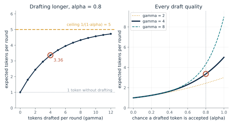
Chance a draft token is accepted (alpha): 0.8 · Tokens drafted (gamma): 4

At alpha = 0.8 and gamma = 4, one round gives 3.36 tokens on average. Raising gamma can never pass 1/(1-alpha) = 5, so each extra drafted token helps less than the one before.

Expected tokens per round: 3.36
Most any gamma can reach: 5
Gain over one token: 2.36 extra
Share of the gamma + 1 maximum: 67.2%

Why it matters for language models

Speculative decoding speeds up generation without changing the output distribution, but the gain depends entirely on how well the small model imitates the large one on the task at hand.

Show the calculation

E = (1 - alpha^(gamma+1)) / (1 - alpha) = (1 - 0.8^5) / (1 - 0.8) = (1 - 0.328) / 0.2 = 3.36.

The equations and symbols

$\mathbb{E}[\text{tokens per round}]=\sum_{k=0}^{\gamma}\alpha^{k}=\frac{1-\alpha^{\gamma+1}}{1-\alpha}$

$\alpha=\sum_x\min(p(x),q(x))=1-\mathrm{TV}(p,q),\qquad \lim_{\gamma\to\infty}\mathbb{E}=\frac{1}{1-\alpha}$

alpha: chance the large model accepts one drafted token
gamma: tokens the draft model proposes per round
p, q: large (target) and small (draft) model distributions
TV: total variation distance between p and q

Where the conclusion applies

Each drafted token is accepted independently with the same chance alpha (the book's approximation). One round counts the accepted prefix plus one token from the large model. Alpha = 1 makes the closed form 0/0; the sum gives gamma + 1. Real speedup also depends on how costly the draft passes are and on available parallelism.

Check your understanding: With alpha = 0.5 and gamma = 3, how many tokens per round, and what is the ceiling?

(1 - 0.5^4)/(1 - 0.5) = 0.9375/0.5 = 1.875 tokens. The ceiling as gamma grows is 1/(1 - 0.5) = 2.

Book source: Chapter 8, 8.10.5 Speculative Decoding and the Acceptance-Rate Analysis; 8.10.6 Worked Example: Acceptance Rate and Expected Speedup. Illustration C08-D05. Identity. Book formula and worked examples: alpha = 0.8 with gamma = 4 gives 3.36, and alpha = 0.4 with gamma = 4 gives 1.65. Other values extend the same formula. v39 EPUB / v43 print.

06 / 08

A built-in penalty for distance

From Chapter 8, 8.2.6 ALiBi; 8.2.7 ALiBi: Mathematical Analysis of Length Bias

How does a straight-line penalty on attention scores turn into smooth decay with distance, and how does each head's slope set its reach?

The score for a pair of tokens loses m times their distance. Inside the exponential, that subtraction becomes a multiplication by exp(-m x distance), a smooth decay. Eight heads use eight slopes spaced by factors of two.

Predict first: Compare the steep head 2 with the shallowest head 8 over 32 tokens. Which head still gives distant tokens most of their weight, and how far away does its factor fall to one half?

Head number (h): 2

18

Tokens shown

Left: lower-triangle heat map of the distance factor, hatched above. Right: decay curves for all eight heads with the chosen head thick. — **Each head's slope sets how far it reaches: steep slopes make a local head, shallow slopes make a broad one.**
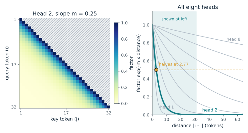
Head number (h): 2 · Tokens shown: 32

Head 2 multiplies each key's weight by exp(-m x distance) with m = 0.25. The factor halves every 2.77 tokens, so this head is strongly local. Content scores also matter after softmax.

Slope of this head (m): 0.25
Factor one token away: 0.779
Distance where the factor halves: 2.77 tokens
Factor 31 tokens away: 0.000431

Why it matters for language models

ALiBi gives each head a different reach, so a model gets both local and long-range views of the text. The penalty is defined for any distance, which is why such models can be run on longer inputs than they trained on, though accuracy there still needs testing.

Show the calculation

m = 2^(-8h/H) = 2^(-8 x 2 / 8) = 2^(-2) = 0.25. Half-distance = ln 2 / m = 0.693 / 0.25 = 2.77 tokens. At distance 31: exp(-0.25 x 31) = 0.000431.

The equations and symbols

$A_{ij}\propto\exp\!\Big(\frac{q_i^\top k_j}{\sqrt{d_k}}-m_h|i-j|\Big)$

$m_h=2^{-8h/H}\quad(h=1,\dots,H),\qquad \text{half-distance}=\frac{\ln 2}{m_h}$

m_h: slope of head h (fixed, not learned)
|i - j|: distance in tokens between query i and key j
h, H: head number and number of heads (8 here)
factor: exp(-m x distance), the distance part of the weight

Where the conclusion applies

The plotted factor is the distance part of the unnormalized weight. In exact softmax attention the shared denominator and the content scores still matter, so decay of the final weights holds only under the book's mean-field approximation. Only keys at or before the query are shown (causal).

Check your understanding: For head 3 (slope 1/8), how many tokens until the factor halves?

ln 2 / 0.125 = 0.693 / 0.125, about 5.5 tokens. Each factor-of-two drop in slope doubles the half-distance.

Book source: Chapter 8, 8.2.6 ALiBi; 8.2.7 ALiBi: Mathematical Analysis of Length Bias. Illustration C08-D06. Identity. Book slope schedule m_h = 2^(-8h/H) with H = 8 heads, as in the book's ALiBi figure; the token counts shown are illustrative. v39 EPUB / v43 print.

07 / 08

Move rounding difficulty from activations to weights

From Chapter 8, 8.14.1 The Rounding-Error Objective; 8.14.4 SmoothQuant: Moving Difficulty from Activations to Weights

One channel has activations up to 20 and weights up to 0.5. How can rescaling make both easier to round to a few bits?

Dividing a channel of activations by s and multiplying the matching weights by s leaves their product unchanged. The rounding step, however, uses one scale for the whole tensor, so one huge channel wastes most of the available levels. Choosing s from both ranges evens them out.

Predict first: At alpha = 0 the outlier makes the activations hard to round. Slide alpha to 0.5. What happens to the two ranges of the outlier channel, and to the overall output error?

Smoothing share (alpha): 0

01

Bits per number

Left: activation, weight and output rounding error against alpha. Right: bars of channel ranges after rescaling, with before-values marked. — **Rescaling by s moves the same product's rounding difficulty from outlier activations onto the weights, and a middle alpha balances them.**
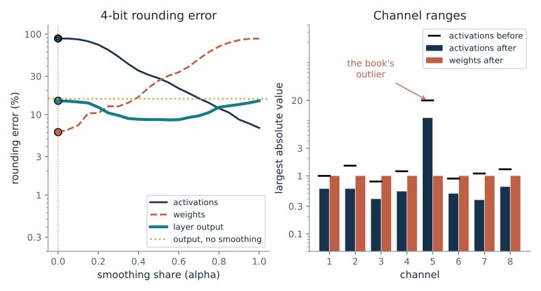
Smoothing share (alpha): 0 · Bits per number: 4

At alpha = 0 the outlier channel's ranges are 10 (activation) and 1 (weight). Raising alpha moves rounding damage from activations to weights, and the full-precision product is unchanged. Activation and weight errors are averages over channels; the output error is lowest in between.

Activation error (average over channels): 88.3%
Weight error (average over channels): 6.06%
Layer output error (whole output): 14.8% (no smoothing: 15.7%)
Outlier channel range after (activation, weight): 10, 1

Why it matters for language models

A handful of outlier channels in activations are what make low-bit quantization of large models hard. Rescaling channels before rounding is one standard way to store and run a model with fewer bits and less memory.

Show the calculation

Outlier channel: s = 20^0 / 0.5^1 = 2. Activation range 20 / 2 = 10; weight range 0.5 x 2 = 1. At alpha = 0.5, s = sqrt(40) = 6.32 and both ranges are 3.16.

The equations and symbols

$s_j=\frac{\max_i|X_{ji}|^{\alpha}}{\max|W_{\cdot j}|^{1-\alpha}},\qquad X'=\operatorname{diag}(s)^{-1}X,\quad W'=W\operatorname{diag}(s)$

$W'X'=WX\ \ \text{exactly (full precision)},\qquad \hat x=s_q\,\mathrm{round}(x/s_q)$

X: activations: one row per channel, one column per token
W: weights: one column per channel
s_j: rescaling factor for channel j
alpha: share of the burden moved to the weights (0 to 1)
bits: bits per stored number after rounding

Where the conclusion applies

A symmetric round-to-nearest quantizer with one scale for each whole tensor and 2^(bits-1) - 1 levels each side (the book's affine quantizer with zero-point 0). Activation and weight errors are the average, over channels, of each channel's own relative rounding error, so a small channel crushed to zero counts fully; the layer output error is relative to the size of the whole output. One toy layer, no calibration data, no outlier exceptions.

Check your understanding: An activation channel reaches 8 and its weights reach 0.5. What are s and the new ranges at alpha = 0.5?

s = sqrt(8) / sqrt(0.5) = 4. The activation range becomes 8/4 = 2 and the weight range 0.5 x 4 = 2.

Book source: Chapter 8, 8.14.1 The Rounding-Error Objective; 8.14.4 SmoothQuant: Moving Difficulty from Activations to Weights. Illustration C08-D07. Simulation. Book worked example: activation channel up to 20, weight column up to 0.5, alpha 0.5, giving s = sqrt(40) = 6.32 and both ranges 3.16. The other seven channels, 64 random tokens (seed 8014) and the quantizer are companion toy choices. v39 EPUB / v43 print.

08 / 08

Penalize uneven expert traffic

From Chapter 8, 8.7.5 Worked Example: MoE Expert Routing Analysis; 8.6.4 Mixture of Experts: Routing Theory and Load Balancing

When a router sends tokens to experts, how does one number tell us the work is uneven?

The loss multiplies, expert by expert, how much traffic it received by how much the router wanted to send it, then sums and scales by the number of experts. Evenly spread traffic and weights give exactly 1. Concentrating both on the same expert drives the sum up.

Predict first: In the book batch, expert 1 gets 3 of 8 tokens and a router weight of 0.4. Is the loss above or below 1, and what value does it take if every token goes to expert 1?

Routing pattern

Share moved to even routing: 0

01

The load-balance loss grows when the experts that receive most tokens are also the ones the router favors, and falls toward 1 as shares even out.
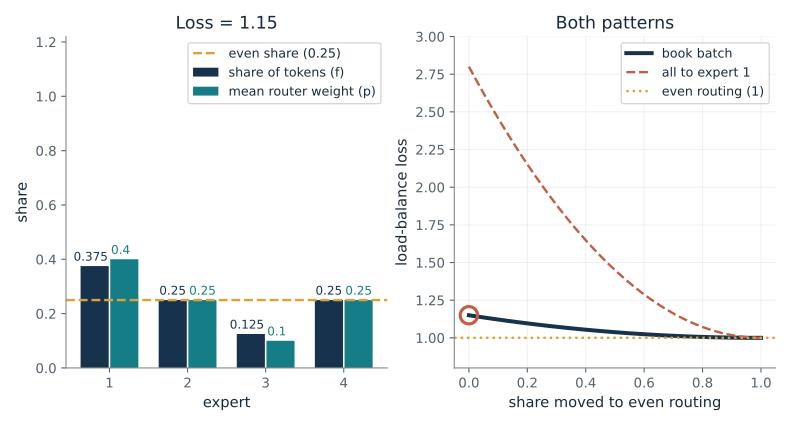
Routing pattern: book batch · Share moved to even routing: 0

The loss is 1.15, above the even-routing value 1. It rises when the experts that receive many tokens are also the ones the router likes most. Moving toward even shares lowers it.

Load-balance loss: 1.15
Loss with perfectly even routing: 1
Excess over even routing: 0.15
Busiest expert's share of tokens: 0.375

Why it matters for language models

Without a penalty like this, a mixture-of-experts layer can collapse to a few popular experts and waste the rest. The loss is added to the training objective to keep all experts in use.

Show the calculation

Loss = E x sum of f x p = 4 x (0.375 x 0.4 + 0.25 x 0.25 + 0.125 x 0.1 + 0.25 x 0.25) = 4 x 0.288 = 1.15.

The equations and symbols

$\mathcal{L}_{\text{load}}=E\sum_{e=1}^{E}f_e\,p_e$

$f_e=\frac{\text{tokens sent to expert }e}{B},\qquad p_e=\text{mean router weight on expert }e$

E: number of experts (4 here)
B: tokens in the batch (8 here)
f_e: share of tokens actually sent to expert e
p_e: average router probability for expert e
L: load-balance loss; 1 for perfectly even routing (also 1 whenever p is uniform, whatever f is)

Where the conclusion applies

Top-1 routing. The blend mixes both f and p with the even value 0.25, so it shows how the formula responds and is not a training trajectory. The loss is 1 for exactly even f and p; for arbitrary unrelated f and p it is not a lower bound, because the Switch loss ties f to the router's own choices.

Check your understanding: With 4 experts, f = (0.5, 0.5, 0, 0) and p = (0.25, 0.25, 0.25, 0.25), what is the loss?

4 x (0.5 x 0.25 + 0.5 x 0.25) = 4 x 0.25 = 1. Even router weights give 1 whatever the traffic split, which is why the penalty acts through both f and p.

Book source: Chapter 8, 8.7.5 Worked Example: MoE Expert Routing Analysis; 8.6.4 Mixture of Experts: Routing Theory and Load Balancing. Illustration C08-D08. Identity. Book worked example: 8 tokens, 4 experts, f = (0.375, 0.25, 0.125, 0.25), p = (0.4, 0.25, 0.1, 0.25), loss 1.15. The collapse pattern and the blend toward even routing are companion extensions. v39 EPUB / v43 print.

Which values reach the current token?

Change variety without confusing it with accuracy

Keep the gap while moving both positions

Count context cost in the right units

How many tokens does one checked draft give?

A built-in penalty for distance

Move rounding difficulty from activations to weights

Penalize uneven expert traffic

Bring the idea to a question of your own