Chapter 9 · Graph and Geometric Deep Learning

01 / 08

A weak bridge lowers graph connectivity

From Chapter 9, 9.1.2 The Graph Laplacian and Its Spectrum

Two groups of three nodes are joined by one bridge. How much connectivity is lost when the bridge is weakened?

The Laplacian charges every disagreement between neighbors. A signal that is -1 on one group and +1 on the other disagrees only across the bridge, so its energy is 4b. Divide by the size of the signal, 6, to get 4b/6. Lambda 2 is the smallest such ratio over all mean-zero signals, so it is at most 4b/6.

Predict first: If the bridge weight is halved from 1 to 0.5, does lambda 2 halve too?

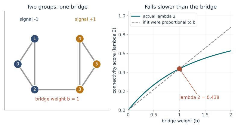
Bridge weight (b): 1

02

Left: two triangles joined by a bridge. Right: lambda 2 rises with bridge weight, below a dashed line of strict proportion. — **Weakening the only bridge lowers lambda 2, reaching exactly 0 when the bridge is gone, but lambda 2 does not fall in proportion to the bridge weight.**
Bridge weight (b): 1

With bridge weight 1, lambda 2 is 0.438. Halve the bridge and compare: the dashed line shows what strict proportion would predict, and the real curve lies above it.

Connectivity score (lambda 2): 0.438
Separate groups: 1
Energy of the two-group signal: 4
Energy divided by size (an upper limit for lambda 2): 0.667

Why it matters for language models

A sparse attention pattern is a graph on tokens, and a small lambda 2 means only weak links join its groups, so information crosses between those groups slowly.

Show the calculation

Only the bridge joins a -1 node to a +1 node, so the signal f = (-1, -1, -1, 1, 1, 1) has energy f^T L f = b x (1 - (-1))^2 = 4b. Here 4 x 1 = 4. The signal has size f^T f = 6, so energy over size is 4 / 6 = 0.667. Lambda 2 is the smallest such ratio over all mean-zero signals, so it is at most this: 0.438 <= 0.667.

The equations and symbols

$L=D-A,\qquad f^\top Lf=\frac12\sum_{i,j}A_{ij}(f_i-f_j)^2$

$\lambda_2=\min_{f\perp\mathbf{1},\ f\ne0}\frac{f^\top Lf}{f^\top f}$

A: adjacency matrix: edge weights between nodes
D: diagonal matrix of each node's total edge weight
L: graph Laplacian, D minus A
f: a number attached to each node (a signal)
lambda 2: connectivity score: second smallest eigenvalue of L; 0 exactly when the graph splits
b: weight of the bridge between nodes 2 and 3

Where the conclusion applies

Two triangles with unit edges joined by one bridge of weight b >= 0. Positive weights determine connectivity. The half factor counts every pair in both orders; a single edge counted once has no half. Weights and signals are dimensionless.

Check your understanding: If the bridge weight is 0.5 and the group signals are -2 and +2, what is the energy f^T L f?

Only the bridge contributes: 0.5 x (2 - (-2))^2 = 8. Counting both directions gives 16 before dividing by two.

Book source: Chapter 9, 9.1.2 The Graph Laplacian and Its Spectrum. Illustration C09-D01. Illustration. Book equation with companion toy graphs stated in the assumptions; every plotted value and worked calculation is recomputed. v39 EPUB / v43 print.

02 / 08

Two ways to normalize, one constant signal

From Chapter 9, 9.2.3 GCN: Graph Convolutional Network

If every node holds the same value, does one round of neighbor mixing leave them all equal?

Each node replaces its value with a weighted sum over itself and its neighbors. Row weights sum to 1 for the row-average rule, so equal inputs stay equal. The symmetric rule divides by both end counts, so a node with many neighbors collects a different total.

Predict first: Start with 1 at every node. After many rounds, which rule still has every node at exactly 1?

Rounds of mixing: 1

012

Rule shown on the graph

Left: six graph nodes colored by value after one round. Right: bars for both rules; the row rule stays at 1, the symmetric rule does not. — **A row-average rule keeps a constant signal constant; the symmetric GCN rule does not, so it is not literally an average.**
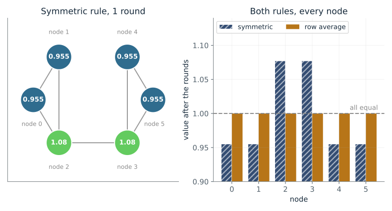
Rounds of mixing: 1 · Rule shown on the graph: symmetric

After 1 round the nodes hold values from 0.955 to 1.08. The symmetric rule is not an average, so the equal signal drifts toward 0.946 on nodes with 2 neighbors and 1.09 on nodes with 3.

Smallest node value: 0.955
Largest node value: 1.08
Gap between them: 0.122
Weight node 0 sends to node 2 each round: 0.289

Why it matters for language models

Attention weights are a softmax whose rows sum to 1, which is the row-average rule; a layer built from symmetric normalization can change the overall scale of a signal instead.

Show the calculation

Count each node together with its neighbors. Node 2 has 3 neighbors, so its count is 4; nodes 0 and 1 have count 3; node 3 has count 4. Row rule: node 2 averages its four entries, each weight 1/4, and 4 x 1/4 = 1. Symmetric rule: weight from node 0 or 1 is 1/sqrt(4 x 3) = 0.289, from node 3 it is 1/sqrt(4 x 4) = 0.25, from itself 0.25. These add to 1.08, not 1, so a constant signal grows at node 2 in one round. After 1 round node 2 holds 1.08 under the symmetric rule and 1 under the row rule.

The equations and symbols

$H^{(\ell+1)}=\sigma(\hat A H^{(\ell)}W^{(\ell)})$

$\hat A=\tilde D^{-1/2}(A+I)\tilde D^{-1/2},\qquad P=\tilde D^{-1}(A+I)$

H: one number per node (here every node starts at 1)
A + I: adjacency plus a self-link at each node
D-tilde: each node's link count including its self-link
A-hat: symmetric rule, used by the GCN
P: row-average rule: each row of weights sums to 1

Where the conclusion applies

The same two-triangle graph with unit bridge and unit self-links. Weights W = 1, no bias and identity activation, so only the normalization acts. Every node starts at 1.

Check your understanding: In a graph where every node has the same number of neighbors, do the two rules differ?

No. If every count is c, the symmetric weight is 1/sqrt(c x c) = 1/c, the same as the row rule. They differ only when counts differ.

Book source: Chapter 9, 9.2.3 GCN: Graph Convolutional Network. Illustration C09-D02. Illustration. Book equation with companion toy graphs stated in the assumptions; every plotted value and worked calculation is recomputed. v39 EPUB / v43 print.

03 / 08

Many rounds erase differences

From Chapter 9, 9.7.1 The Depth-Smoothness Trade-off

If a signal is mixed with its neighbors over and over, do all node values become equal?

Every mixing round shrinks all parts of the signal except one. The part that survives follows the square root of each node's link count. Distinctions that depend on the shrinking parts fade by about a factor rho per round.

Predict first: After 32 rounds, will all six values be equal?

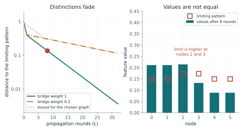
Mixing rounds (L): 8

132

Bridge weight

After 8 rounds the values are 0.136 away from the limiting pattern, under the bound 0.277. That pattern is not equal across nodes: it is 0.15 at nodes with 2 neighbors and 0.173 at nodes with 3. A weaker bridge keeps rho closer to 1, so the fade is slower.

Slowest shrink factor per round (rho): 0.86
Distance to the limit now: 0.136
Upper bound: 0.277
Limit at nodes 0 and 2: 0.15 and 0.173

Why it matters for language models

Token representations in a deep stack of mixing layers can become too alike; here the same pull toward a common pattern is exact and its speed is a number, rho.

Show the calculation

The slowest shrink factor is rho = 0.8604 and the starting distance is 0.922. After 8 rounds the bound rho^L x (starting distance) is 0.277. The measured distance 0.136 is below it. The limiting value at each node is proportional to the square root of (neighbors + 1), which is not the same for every node, so raw values stay unequal.

The equations and symbols

$H^{(L)}=\hat A^L H^{(0)},\qquad H^*=vv^\top H^{(0)}$

$\|H^{(L)}-H^*\|_2\leq\rho^L\|H^{(0)}-H^*\|_2$

L: number of mixing rounds
H(0): starting values: 1 at node 0, 0 elsewhere
v: unit vector proportional to the square root of each node's link count
H*: limiting pattern the values approach
rho: slowest shrink factor per round (0 to 1)

Where the conclusion applies

Connected undirected graph, positive bridge weight, unit self-links, identity activation and unit weights. The computed rho is below 1, and the Euclidean norm of the one-feature signal equals the Frobenius norm.

Check your understanding: If rho = 0.8 and the starting distance is 2, what does the bound guarantee after three rounds?

The distance is at most 2 x 0.8^3 = 1.024. It is only an upper bound; the real distance can be smaller.

Book source: Chapter 9, 9.7.1 The Depth-Smoothness Trade-off. Illustration C09-D03. Illustration. Book equation with companion toy graphs stated in the assumptions; every plotted value and worked calculation is recomputed. v39 EPUB / v43 print.

04 / 08

Local labels can miss global structure

From Chapter 9, 9.3.1 The 1-WL Test

Can the Weisfeiler-Lehman (WL) test, which relabels each node from its neighbors' labels, tell a six-cycle from two triangles?

Every node starts with the same label and sees two neighbors with that label, so its signature never changes. Marking one node gives the test something to spread, and the two graphs spread it differently.

Predict first: Starting from identical labels, will extra rounds ever tell the cycle from the triangles? What if one node is marked?

Relabeling rounds: 2

05

Starting labels

A six-cycle and two triangles, every node the same color class A, although one graph is connected and the other has two pieces. — **With identical starting labels the WL test sees the same thing in a six-cycle and in two triangles, though one is connected and the other is not.**
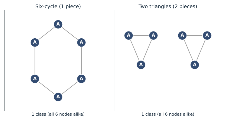
Relabeling rounds: 2 · Starting labels: all the same

After 2 rounds both graphs still have one class: every node sees two neighbors with the same label as its own. The test cannot tell one connected loop from two separate triangles.

Classes in the six-cycle: 1
Classes in the two triangles: 1
Class sizes agree: yes
Connected pieces: 1 and 2

Why it matters for language models

Message-passing layers cannot separate nodes that this test cannot, which is why graph transformers add positional information; a marked node here plays the role of a position.

Show the calculation

Each node reads its own label and the sorted labels of its neighbors, then all signatures are renamed with one shared list. Every node in both graphs reads (own label, [same, same]), so all twelve nodes get one shared new label and the counts agree at every round.

The equations and symbols

$c_{t+1}(v)=\mathrm{HASH}\left(c_t(v),\{\!\{c_t(u):u\in N(v)\}\!\}\right)$

c_t(v): label (color class) of node v after t rounds
N(v): the neighbors of v
{{ }}: a multiset: repeats are kept, order is ignored
HASH: a shared lookup that gives equal signatures the same new label

Where the conclusion applies

Both six-node graphs are unweighted and start with the same labels. One shared relabeling is used for both graphs. Stable means the partition into classes stops changing, not that the color names match.

Check your understanding: If every node of both graphs gets its own unique ID, can the test tell them apart?

Yes. Unique IDs give every node a different class at the start. The blindness result only holds when starting labels are identical, so it cannot be reused for the new setup.

Book source: Chapter 9, 9.3.1 The 1-WL Test. Illustration C09-D04. Illustration. Book equation with companion toy graphs stated in the assumptions; every plotted value and worked calculation is recomputed. v39 EPUB / v43 print.

05 / 08

A small eigenvalue guarantees a bottleneck

From Chapter 9, 9.1.5 The Cheeger Inequality and Graph Expansion

The weakest cut of a graph is hard to find. What does an easy eigenvalue tell us about it?

The cut score asks, for the weakest way to split the graph, how much edge weight crosses compared with the smaller side. The eigenvalue is quick to compute and always sits within a fixed band of that score. In this graph the best cut is one triangle against the other.

Predict first: As the bridge gets very weak, does the weakest-cut score stay nearer the lower end or the upper end of the band the theorem allows?

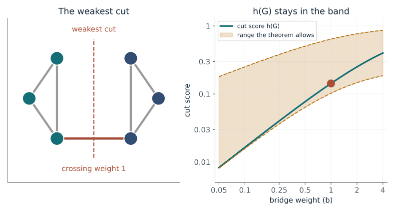
Bridge weight (b): 1

0.054

Left: two triangles with the weakest cut drawn through the bridge. Right: the cut score runs inside a shaded band set by the eigenvalue. — **The weakest-cut score always lies between lambda-tilde 2 / 2 and sqrt(2 lambda-tilde 2), so a tiny eigenvalue proves a bottleneck exists.**
Bridge weight (b): 1

With bridge weight 1, the weakest cut scores 0.143. The theorem puts it between 0.102 and 0.64; here it sits inside the band. The eigenvalue is not small here, so the band is wide and the bottleneck is mild.

Second eigenvalue (lambda-tilde 2): 0.205
Weakest-cut score h(G): 0.143
Lower end of the band: 0.102
Upper end of the band: 0.64

Why it matters for language models

Spectral clustering of embedding vectors uses this link: the second eigenvector finds a cut that the inequality says is nearly as good as the best one.

Show the calculation

Best cut: one triangle on each side. Crossing weight = b = 1. Each side has volume 2 + 2 + (2 + b) = 6 + b = 7. So h(G) = 1 / 7 = 0.143. Half of lambda-tilde 2 is 0.102 and the square root of 2 x lambda-tilde 2 is 0.64, so lower <= h(G) <= upper.

The equations and symbols

$h(S)=\frac{\sum_{(i,j)\in E(S,\bar S)}A_{ij}}{\min(\mathrm{vol}(S),\mathrm{vol}(\bar S))},\qquad h_G=\min_S h(S)$

$\frac{\tilde\lambda_2}{2}\le h_G\le\sqrt{2\tilde\lambda_2}$

S: one side of a cut (a group of nodes)
vol(S): sum of the degrees of the nodes in S
h(G): cut score of the weakest cut: crossing weight over the smaller volume
lambda-tilde 2: second smallest eigenvalue of the normalized Laplacian

Where the conclusion applies

Two unit triangles joined by one bridge of weight b, no self-links. The normalized Laplacian is I - D^(-1/2) A D^(-1/2). The cut score uses every nonempty proper subset and the smaller of the two volumes.

Check your understanding: A graph has lambda-tilde 2 = 0.02. Between what values must its weakest-cut score lie?

Between 0.02 / 2 = 0.01 and sqrt(2 x 0.02) = 0.2. A small eigenvalue therefore guarantees a cut with score at most 0.2.

Book source: Chapter 9, 9.1.5 The Cheeger Inequality and Graph Expansion. Illustration C09-D05. Identity. Book equation with companion toy graphs stated in the assumptions; every plotted value and worked calculation is recomputed. The cut score is found by trying all 62 ways to split the six nodes. v39 EPUB / v43 print.

06 / 08

Curvature finds the bottleneck edge

From Chapter 9, 9.11.3 Computing Ollivier-Ricci Curvature: Path Graph P4 (with 9.4.3)

Can a single number per edge show which links are bottlenecks and which sit inside tight groups?

Each node spreads probability evenly over its neighbors. If the two spreads overlap a lot, little has to move and curvature is high. If they are far apart, a lot moves and curvature drops, below zero once the cost exceeds the edge length.

Predict first: In the path graph P4, which edge is the most curved?

Graph

Edge to inspect

Left: two triangles with a thick red bridge labeled -2/3 and teal triangle edges labeled positive. Right: bars of the two neighbor spreads. — **Curvature separates edges inside tight groups (positive) from a bridge between groups (negative); a path and a four-cycle are flat in this measure.**
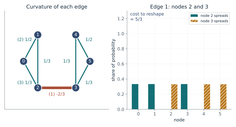
Graph: two triangles + bridge · Edge to inspect: 1

Edge 2-3 has curvature -2/3, negative: the two neighborhoods are far apart, the signature of a bottleneck.

Curvature of this edge: -2/3
Cost to reshape one cloud into the other: 5/3
Lowest curvature in this graph: -2/3
Edges with negative curvature: 1 of 7

Why it matters for language models

Rewiring methods add links where curvature is most negative; the same idea of adding shortcuts where information is squeezed motivates global tokens and long-range links in sparse-attention models.

Show the calculation

Node 2 spreads its probability evenly over its neighbors: 1/3 at node 0, 1/3 at node 1, 1/3 at node 3. Node 3: 1/3 at node 2, 1/3 at node 4, 1/3 at node 5. The cheapest way to reshape one into the other moves mass a total distance of 5/3. Curvature = 1 - 5/3 = -2/3, since the edge length is 1.

The equations and symbols

$\kappa(i,j)=1-\frac{W_1(\mu_i,\mu_j)}{d_G(i,j)}$

$\mu_i(k)=\frac{A_{ik}}{\sum_m A_{im}},\qquad \kappa(i,j)=1-W_1(\mu_i,\mu_j)\ \ \text{when } d_G(i,j)=1$

mu_i: spread of probability evenly over the neighbors of node i
W1: cheapest total distance to reshape one spread into the other
kappa: edge curvature: positive if the spreads overlap, negative if far apart
d: shortest-path distance between two nodes

Where the conclusion applies

Small unweighted graphs, no lazy step, hop distance. Curvature is a diagnostic: the book stresses that it does not by itself give a sensitivity bound. Edges are numbered in the order of the plot labels (1) to (3); nodes are numbered from 0, as in the other demos.

Check your understanding: In the complete graph K4 each pair of connected nodes shares two neighbors. Is its curvature positive, zero or negative?

Positive, 2/3. Node 0 spreads over nodes 1, 2, 3 and node 1 over nodes 0, 2, 3. Two thirds of the mass already overlaps, so only 1/3 moves, at cost 1/3.

Book source: Chapter 9, 9.11.3 Computing Ollivier-Ricci Curvature: Path Graph P4 (with 9.4.3). Illustration C09-D06. Illustration. Book equation with companion toy graphs stated in the assumptions; every plotted value and worked calculation is recomputed. W1 is solved exactly as a small transport problem. v39 EPUB / v43 print.

07 / 08

Over-squashing: distant inputs barely arrive

From Chapter 9, 9.4.2 Formal Sensitivity Analysis

At the same distance, how much more of a far-away input reaches a node on a grid than on two cliques joined by a thin chain?

The coefficient adds up weights over all routes of exactly L steps. A grid has many routes of the same length. The barbell has one, and each step through a big clique is divided by that clique's size.

Predict first: At the same distance L, does the barbell pass more or less of the source signal than the grid?

Distance and layers (L): 5

38

Clique size

Left: two cliques joined by a chain with source and target marked. Right: log plot where the barbell curve lies far below the grid curve. — **At equal distance the barbell's coefficient is far smaller than the grid's, and the gap widens with bigger cliques and longer chains.**
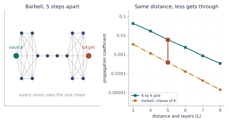
Distance and layers (L): 5 · Clique size: 6

At distance 5 the grid passes 15.5 times more than the barbell: 0.00584 against 0.000378. The barbell has one narrow chain that every route must use, so a far-away input barely reaches the target. Most of the steps are chain steps, each weighted 1/3.

Coefficient on the barbell: 0.000378
Coefficient on the grid: 0.00584
Grid divided by barbell: 15.5x
Nodes in the barbell: 14

Why it matters for language models

Long-range information is hard to carry through a narrow path; in sequence models a fixed-size state or a thin chain of layers faces the same squeeze.

Show the calculation

The coefficient is the (target, source) entry of A-hat^L with L = 5. Only one shortest route exists on the barbell, and each step is weighted by 1/sqrt(a x b) for the entry counts at its two ends. Computed: barbell 0.000378, grid 0.00584, ratio 15.5.

The equations and symbols

$\left|\frac{\partial h_i^{(L)}}{\partial x_s}\right|\le(\alpha\beta)^L\,[\hat A^L]_{is}$

h_i(L): representation of node i after L layers
x_s: input at the source node s
alpha, beta: bounds on the layer's slopes (taken as 1 here)
[A-hat^L]_is: propagation coefficient: row i, column s of the L-th power of the symmetric rule

Where the conclusion applies

Barbell: two cliques joined through a chain, with source and target at the far corners, L steps apart. Grid: 6 by 6, the target L steps from a corner. Self-links added, symmetric normalization. The coefficient is a propagation coefficient, not generally a probability, and it bounds sensitivity only under the lemma's assumptions.

Check your understanding: On a path graph where every inner node has 2 neighbors (count 3 with the self-link), what factor does one extra chain step multiply the coefficient by?

1/3. Each extra step crosses a node pair with counts 3 and 3, so the weight is 1/sqrt(3 x 3) = 1/3. This matches the barbell values, which fall by a factor of 3 per step.

Book source: Chapter 9, 9.4.2 Formal Sensitivity Analysis. Illustration C09-D07. Illustration. Book equation with companion toy graphs stated in the assumptions; every plotted value and worked calculation is recomputed. This is the coefficient in the book's upper bound, not a measured sensitivity. v39 EPUB / v43 print.

08 / 08

A filter built from repeated multiplication

From Chapter 9, 9.5.2 ChebNet (with 9.1.4)

How can a graph network apply a frequency filter without computing any eigenvectors?

Multiplying by the Laplacian mixes neighbors once. A polynomial of degree K in the Laplacian therefore mixes up to K hops, yet equals a filter on the frequencies. The Chebyshev recurrence builds each term from the previous two, so no eigenvectors are ever needed.

Predict first: How many matrix-vector products does the smooth filter exp(-lambda) need to be accurate within 1% on this graph?

Polynomial degree (K): 2

012

Wanted filter

Left: a sharp low-pass target and its dashed degree-2 polynomial, with the six graph frequencies marked. Right: input, exact and filtered signals. — **A low-degree polynomial in the Laplacian filters the graph signal accurately where it counts, at the graph's own frequencies, using only repeated multiplication.**
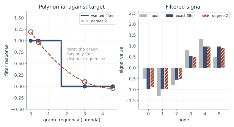
Polynomial degree (K): 2 · Wanted filter: sharp low-pass

At the graph's own six frequencies the degree 2 response is off by at most 0.19, and the filtered signal is off by 5.32%. Only those few frequencies matter, not the whole curve. A sharp cutoff needs many terms and wiggles.

Polynomial degree (K): 2
Matrix-vector products used: 2
Largest error at the six frequencies: 0.19
Error in the output signal: 5.32%

Why it matters for language models

Each extra degree is one more hop of message passing, so a degree-K filter is a K-hop layer; this ties spectral filtering to the local update rule in GCNs.

Show the calculation

The filter is the sum from k = 0 to 2 of theta_k T_k(L-tilde), where L-tilde = 2L/4.56 - I. It is applied with the recurrence T_k = 2 L-tilde T_(k-1) - T_(k-2), which takes 2 matrix-vector products and never finds eigenvectors. The weights theta_k here are the first Chebyshev series coefficients of the wanted filter (a trained ChebNet learns them instead): 0.418, -0.616, 0.157.

The equations and symbols

$g_\theta(\tilde L)=\sum_{k=0}^{K}\theta_kT_k(\tilde L),\qquad \tilde L=\frac{2L}{\lambda_{\max}}-I$

$T_0=1,\quad T_1=x,\quad T_k=2xT_{k-1}-T_{k-2}$

lambda: graph frequency: an eigenvalue of the Laplacian L
g(lambda): response of the wanted filter at frequency lambda
T_k: Chebyshev polynomial of degree k
theta_k: weight on T_k (learned in ChebNet; set from the wanted filter here)
K: polynomial degree = number of matrix-vector products

Where the conclusion applies

The two-triangle graph with unit bridge (Laplacian eigenvalues 0, 0.438, 3, 3, 3, 4.56). Wanted filters: exp(-lambda), or 1 up to lambda = 1.7 and 0 above. A trained ChebNet would learn theta_k from data. Only the six eigenvalues matter for this graph.

Check your understanding: With degree K = 0, what does the filter do to a signal?

It only rescales the signal by theta_0 and mixes no neighbors. Every frequency gets the same response, so no frequency is removed.

Book source: Chapter 9, 9.5.2 ChebNet (with 9.1.4). Illustration C09-D08. Illustration. Book equation with companion toy graphs stated in the assumptions; every plotted value and worked calculation is recomputed. Fixed signal: (-1, -1, -1, 1, 1, 1) plus a small jitter. Weights are the leading Chebyshev series coefficients of the wanted filter. v39 EPUB / v43 print.

A weak bridge lowers graph connectivity

Two ways to normalize, one constant signal

Many rounds erase differences

Local labels can miss global structure

A small eigenvalue guarantees a bottleneck

Curvature finds the bottleneck edge

Over-squashing: distant inputs barely arrive

A filter built from repeated multiplication

Bring the idea to a question of your own