Chapter 10 · Latent, Adversarial, and Flow Models

01 / 08

Hidden variables make visible variation

From Chapter 10, 10.1.1 The Generative Model and the Intractability of Likelihood

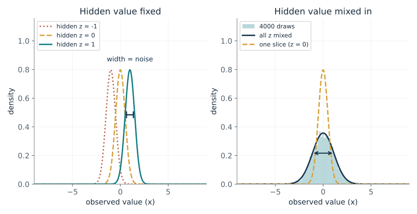
A model first draws a hidden value z, then adds measurement noise. How much of the spread you see comes from the hidden value, and how much from the noise?

Each curve on the left holds z fixed, so only the noise is left. Averaging those curves over all z gives the wider curve on the right, because the hidden value moves the centre. Writing Z as a fixed source E, as in Z = 0 + 1 x E, puts the randomness in one standard place.

Predict first: If the noise stays the same and the gain doubles, does the variance of each slice change?

Hidden-value gain (g): 1

0.53

Observation noise SD (tau)

Left: three narrow bell curves for hidden values -1, 0, 1. Right: one wide bell curve of all draws with a narrow dashed slice inside. — **Fixing the hidden value leaves only the noise variance; letting it vary adds gain squared on top.**
Hidden-value gain (g): 1 · Observation noise SD (tau): 0.5

Each slice has variance 0.25, which is observation noise alone. Letting the hidden value vary adds gain squared, 1, so all draws together have variance 1.25; 80% of it comes from the hidden value.

Variance of one slice: 0.25
Variance of everything: 1.25
Share from the hidden value (%): 80
Variance of the 4000 draws: 1.27

Why it matters for language models

A variational autoencoder generates by drawing a hidden code and decoding it, so the variety in its outputs comes from the code and from the decoder noise together, and the training objective must keep the two apart.

Show the calculation

Conditional variance = noise^2 = 0.5^2 = 0.25. Marginal variance = gain^2 + noise^2 = 1^2 + 0.5^2 = 1 + 0.25 = 1.25. Sampling: Z = 0 + 1 x E with E standard normal, then X = gain Z + noise E2.

The equations and symbols

$p(x)=\int p(x\mid z)p(z)\,dz,\qquad Z=\mu+\sigma E$

$X=gZ+\tau E_2,\qquad \mathrm{Var}(X)=g^2+\tau^2$

X: the value you observe
Z: the hidden value, a standard normal draw
g: gain: how strongly the hidden value moves X
tau: noise SD: the spread added on top of g Z
E, E2: independent standard normal sources of randomness

Where the conclusion applies

Gaussian prior N(0,1) and independent Gaussian observation noise. The 4000 draws use seed 1001 and are illustrative; the curves are exact densities. X has no units.

Check your understanding: For gain 3 and noise SD 0.25, what share of the total variance comes from the hidden value?

The total is 9 + 0.0625 = 9.0625 and the hidden part is 9, so the share is 9 / 9.0625, about 99.3%.

Book source: Chapter 10, 10.1.1 The Generative Model and the Intractability of Likelihood. Illustration C10-D01. Illustration. Book mathematical principle with explicitly defined companion toy inputs; plotted values and worked calculations are recomputed. v39 EPUB / v43 print.

02 / 08

A lower bound and its posterior gap

From Chapter 10, 10.1.2 The Evidence Lower Bound

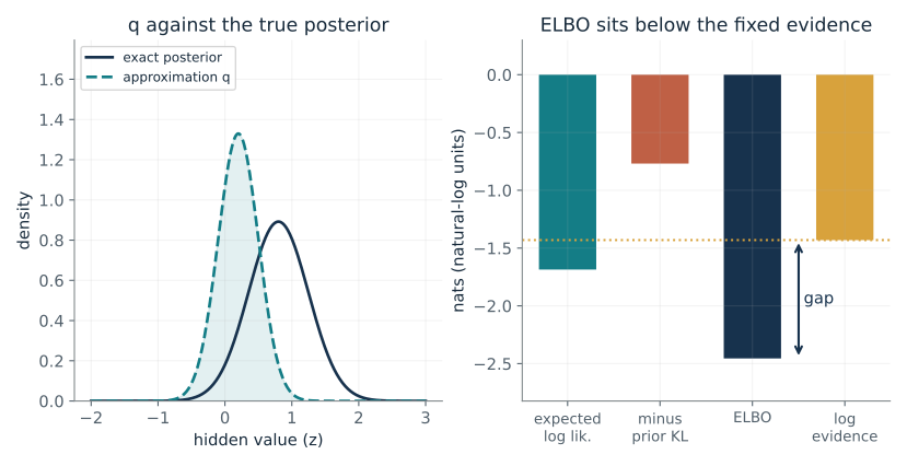
The ELBO is a score that can never exceed the true log evidence. How far below is it, and what controls the distance?

The log evidence cannot be changed by choosing q. The ELBO splits it into a score for q and a leftover gap, the KL distance from q to the exact posterior. Matching the posterior closes the gap; any other width or centre, narrower or wider, opens it.

Predict first: Will making q wider always improve the ELBO?

Centre of q: 0.2

01.5

SD of q

Left: exact posterior and a left-shifted narrow q. Right: bars for log likelihood, prior KL, ELBO and log evidence, with the gap marked. — **The evidence is fixed; the ELBO falls short of it by exactly the distance between q and the true posterior.**
Centre of q: 0.2 · SD of q: 0.3

The approximation q misses the exact posterior (mean 0.8, SD 0.447), so the gap is 1.02. The ELBO is -2.46 against a fixed log evidence of -1.43; the prior KL, 0.769, does not have to be 0.

Prior KL: 0.769
ELBO: -2.46
Log evidence (fixed): -1.43
Gap (KL from q to the posterior): 1.02

Why it matters for language models

Variational autoencoders are trained by raising the ELBO. A high ELBO means a good model only if q is also close to the true posterior, so the gap is the number to watch when judging the approximation.

Show the calculation

Expected log likelihood = -0.5 ln(2 pi x 0.25) - ((1 - 0.2)^2 + 0.3^2)/(2 x 0.25) = -1.69. Prior KL = 0.5 (0.2^2 + 0.3^2 - 1 - ln 0.3^2) = 0.769. ELBO = -1.69 - 0.769 = -2.46. Log evidence = ln N(1; 0, 1.25) = -1.43.

The equations and symbols

$\log p(x)=\mathrm{ELBO}+D_{\mathrm{KL}}(q(z\mid x)\|p(z\mid x))$

$\mathrm{ELBO}=\mathbb E_q\log p(x\mid z)-D_{\mathrm{KL}}(q(z\mid x)\|p(z))$

x: the observed value, fixed at 1
q: the approximate belief about z, a bell curve with chosen centre and SD
p(z | x): the exact belief about z after seeing x: centre 0.8, SD 0.447
KL: a distance-like score between two curves, in nats (natural-log units)
log p(x): log evidence, fixed by the model, here -1.43

Where the conclusion applies

Prior Z ~ N(0,1), likelihood X given Z ~ N(Z, 0.25), x = 1. Only q changes. Widths are positive. Reconstruction is the expected log likelihood, not a raw squared error, and the prior KL is subtracted.

Check your understanding: Which q closes the gap in this example, and does its prior KL become zero?

q = N(0.8, 0.2), SD 0.447. The gap becomes 0 and the ELBO equals the log evidence, but the prior KL stays positive (0.725).

Book source: Chapter 10, 10.1.2 The Evidence Lower Bound. Illustration C10-D02. Illustration. Book mathematical principle with explicitly defined companion toy inputs; plotted values and worked calculations are recomputed. v39 EPUB / v43 print.

03 / 08

Separation and dropped modes

From Chapter 10, 10.4.2 The Wasserstein-1 Distance; 10.4.1 Problems with JS Divergence

What can a transport distance see when the Jensen-Shannon divergence (JS) has stopped changing?

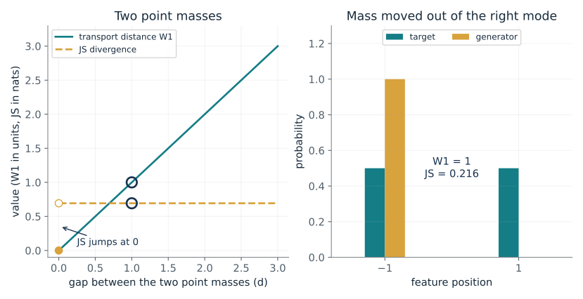
Two separate point masses share no support, so JS can only say they differ. Transport distance charges the amount of probability moved times the distance it travels. A missing mode therefore has a visible cost.

Predict first: If the gap grows from 1 to 2, which comparison doubles?

Gap between point masses (d): 1

03

Mass moved out of the right mode

Left: straight W1 line against a flat JS line at 0.693 with a jump at zero. Right: target bars at -1 and +1 against a generator bar at -1. — **JS saturates at 0.693 once two distributions stop overlapping, while transport distance keeps growing with the gap.**
Gap between point masses (d): 1 · Mass moved out of the right mode: 0.5

At gap 1, JS is stuck at 0.693 (it would say the same at any gap above 0) while W1 reads 1. Moving 0.5 of the mass out of the right mode costs W1 = 1 and leaves the right mode 0% covered (it holds 0 of the mass against the target 0.5).

JS, two point masses (nats): 0.693
W1, two point masses: 1
JS, two modes (nats): 0.216
W1, two modes: 1

Why it matters for language models

A generator trained against a saturated score gets no signal about how far it is from the data; transport-style distances such as the one in Wasserstein GANs keep a usable signal and also charge for a dropped mode.

Show the calculation

Point masses: W1 = d = 1; JS = ln 2 = 0.693 for every d > 0. Two modes: move mass 0.5 a distance 2, so W1 = 0.5 x 2 = 1. JS uses the midpoint m = (p + q)/2: JS = 0.216.

The equations and symbols

$\mathrm{JS}(\delta_0,\delta_d)=\begin{cases}0&d=0\\\log 2&d>0\end{cases},\qquad W_1(\delta_0,\delta_d)=d$

$W_1(p,q)=\inf_\gamma\mathbb E_\gamma|X-Y|$

d: gap between two point masses, in feature units
JS: Jensen-Shannon divergence, in nats
W1: transport distance: probability moved times distance moved
two modes: a target with half its mass at -1 and half at +1

Where the conclusion applies

Exact discrete probabilities and absolute-distance transport cost. JS jumps at d = 0 instead of rising smoothly. The right panel is a separate explicit two-mode example.

Check your understanding: The target has half its mass at -1 and half at +1. A generator puts everything at -1. What is W1?

Half the mass must move a distance 2, so W1 = 0.5 x 2 = 1 feature unit. The right mode has zero coverage.

Book source: Chapter 10, 10.4.2 The Wasserstein-1 Distance; 10.4.1 Problems with JS Divergence. Illustration C10-D03. Illustration. Book mathematical principle with explicitly defined companion toy inputs; plotted values and worked calculations are recomputed. v39 EPUB / v43 print.

04 / 08

Stretching changes density, not mass

From Chapter 10, 10.6.1 The Change-of-Variables Formula

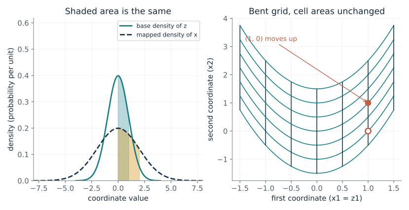
A stretched curve is lower. Where did the probability go?

The inverse map says which base point produced each output. The absolute Jacobian converts between base length and output length. The bent grid shows a nonlinear map whose cell areas stay fixed even though the shapes change.

Predict first: If a = -2, does the density denominator become negative?

Scale of the stretch (a): 2

-24

Bend of the 2D shear (c)

Left: a tall base bell curve and a wider, lower mapped curve with equal shaded areas. Right: a grid bent into parabolas. — **Stretching spreads the same probability over a wider range, so density falls by the scale factor while mapped intervals keep their mass.**
Scale of the stretch (a): 2 · Bend of the 2D shear (c): 1

Scale 2 stretches the curve, so the peak falls to 0.199. The interval z in [0, 1] maps to [0, 2] and keeps mass 0.341.

Total probability: 1
Mass of the mapped interval: 0.341
Mapped interval: [0, 2]
Peak density: 0.199

Why it matters for language models

Normalizing flows give exact likelihoods by tracking this area factor layer by layer; a layer that is not invertible, or has zero scale, would make the likelihood undefined.

Show the calculation

p_X(x) = p_Z((x - 0)/2) / |2|. At x = 0: 0.399 / 2 = 0.199. Mass of z in [0, 1] = Phi(1) - Phi(0) = 0.841 - 0.5 = 0.341. The shear x2 = z2 + 1 z1^2 has Jacobian [[1, 0], [2 z1, 1]], determinant 1, so areas and probabilities are kept.

The equations and symbols

$X=aZ+b,\quad a\ne0,\qquad p_X(x)=\frac{p_Z((x-b)/a)}{|a|}$

$x_1=z_1,\quad x_2=z_2+cz_1^2,\quad \det J=1,\quad p_X(x)=p_Z(x_1,x_2-cx_1^2)$

Z: a standard normal draw
a: scale of the stretch; negative values flip left to right; 0 is not allowed
b: shift (0 here)
c: bend of the 2D shear
det J: area factor of the map; 1 means areas are kept

Where the conclusion applies

Invertible affine map in one dimension, with nonzero scale including a negative value. Total probability is integrated over the whole real line, not read from the plotting window. The 2D shear is invertible for every finite bend and keeps area; no trained flow is implied.

Check your understanding: Map z in [0, 1] using a = -2 and b = 3. What interval and mass result?

The endpoints are 3 and 1, so the image is [1, 3]. Its mass is Phi(1) - Phi(0), about 0.341, despite the reversal.

Book source: Chapter 10, 10.6.1 The Change-of-Variables Formula. Illustration C10-D04. Illustration. Book mathematical principle with explicitly defined companion toy inputs; plotted values and worked calculations are recomputed. v39 EPUB / v43 print.

05 / 08

The best discriminator and the GAN value

From Chapter 10, 10.3.1 The Minimax Formulation

In a GAN the discriminator tries to tell real from generated. What is its best possible score, and what is the generator then minimizing?

At each point the discriminator just reports the fraction of traffic that is real. Putting that best score back into the game leaves a constant plus twice the JS divergence. The generator wins only when the two curves coincide.

Predict first: When the generator matches the data exactly, what does the best discriminator output?

Generator centre (mu): 2

04

Generator SD (sigma)

Left: real data bell curve at 0 and a dashed generator bell curve at 2. Right: a falling S-shaped best-discriminator curve against grey alternatives. — **Against the best discriminator the generator is minimizing twice the JS divergence, and the game value cannot go below -log 4.**
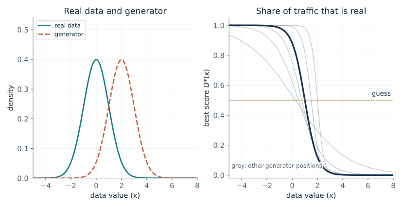
Generator centre (mu): 2 · Generator SD (sigma): 1

The best discriminator scores near 1 where only real data lives and near 0 where only the generator does. The game value -0.712 is 0.674 above the floor, which is twice the JS divergence 0.337.

Game value V (best discriminator): -0.712
Floor, minus log 4: -1.386
Jensen-Shannon divergence (nats): 0.337
Best score at x = 0: 0.881

Why it matters for language models

This is why a GAN generator can stall when the discriminator is too good: far from the data, D* sits at 0 or 1 and the JS score is flat, a gradient problem seen in GAN training.

Show the calculation

D*(x) = p_data(x) / (p_data(x) + p_gen(x)); at x = 0 this is 0.881. V = -log 4 + 2 JS = -1.386 + 2 x 0.337 = -0.712.

The equations and symbols

$D^*(x)=\frac{p_{\mathrm{data}}(x)}{p_{\mathrm{data}}(x)+p_\theta(x)}$

$V(G,D^*)=-\log 4+2\,D_{\mathrm{JS}}(p_{\mathrm{data}}\|p_\theta)$

D*(x): best score at x: the share of traffic there that is real
p_data: density of real data, a standard normal here
p_gen: density of generated data, a bell curve with centre mu and SD sigma
V: the game value the discriminator pushes up and the generator pushes down
JS: Jensen-Shannon divergence, in nats

Where the conclusion applies

Real data N(0,1) and a Gaussian generator. V and JS are computed by numerical integration over a wide grid, each from its own definition; the match V = -log 4 + 2 JS is a result, not an input. Natural logs, so values are in nats.

Check your understanding: The generator is far from the data, so the two curves barely overlap. Roughly what is V?

JS approaches ln 2 = 0.693, so V approaches -1.386 + 2 x 0.693 = 0. The game value is near its ceiling and flat in the generator position.

Book source: Chapter 10, 10.3.1 The Minimax Formulation. Illustration C10-D05. Identity. Book mathematical principle with explicitly defined companion toy inputs; plotted values and worked calculations are recomputed. v39 EPUB / v43 print.

06 / 08

More samples tighten the bound

From Chapter 10, 10.2.1 The Importance-Weighted ELBO

The importance-weighted bound averages M weights before taking the log. How fast does it climb toward the true log evidence?

A single weight is a noisy estimate of the evidence, and the log of a noisy estimate is biased low. Averaging M weights shrinks the noise, so the bias shrinks too. A proposal that is already exact makes every weight equal, so nothing is left to average out.

Predict first: If you keep adding samples, can the bound ever rise above the true log evidence?

Samples averaged (M): 4

164

Proposal q

Left: three bound curves rising with M toward a log evidence line, selected point circled. Right: wide M=1 histogram and narrow M=4 histogram. — **Each extra sample raises the bound toward the log evidence, and it never crosses it.**
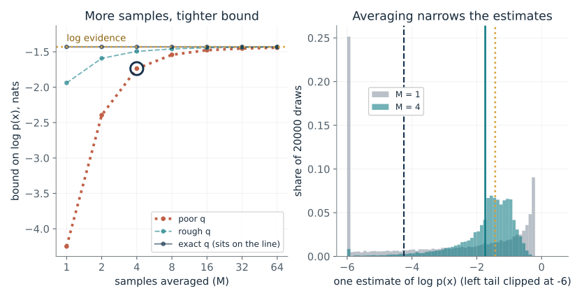
Samples averaged (M): 4 · Proposal q: poor

With M = 4 samples the bound is -1.74, up from the single-sample ELBO -4.25. It stays below the log evidence -1.43, with 0.31 still to close.

Bound with M samples: -1.74
Standard ELBO (M = 1): -4.25
Log evidence: -1.43
Gap left: 0.307

Why it matters for language models

Models trained with this bound get a better likelihood estimate from the same encoder at the cost of M decoder passes per example, a direct compute-for-accuracy trade.

Show the calculation

Bound = average over draws of ln((1/M) sum of weights), weight = p(x|z) p(z) / q(z). M = 1 gives the ELBO -4.25; M = 4 gives -1.74. 20000 seeded draws of up to 64 codes each; log evidence = ln N(1; 0, 1.25) = -1.43.

The equations and symbols

$\mathcal L_M=\mathbb E\left[\log\frac1M\sum_{m=1}^M\frac{p(x\mid z_m)p(z_m)}{q(z_m\mid x)}\right]$

$\log p(x)\ge\mathcal L_{M+1}\ge\mathcal L_M\ge\mathcal L_1=\mathrm{ELBO}$

M: number of hidden codes sampled from q and averaged
weight: p(x | z) p(z) / q(z): how well a code explains x, corrected for how q proposed it
L_M: the bound with M samples, in nats
poor, rough, exact: proposals: N(0,1), mean 0.5 and SD 0.7, and the exact posterior with mean 0.8 and variance 0.2 (SD 0.447)

Where the conclusion applies

Same toy model as the ELBO demo: prior N(0,1), likelihood N(z, 0.25), x = 1. The expectation is estimated from 20000 seeded batches (seed 2026) of up to 64 codes, so values carry a small simulation error. The bound converges to the evidence only when the proposal covers the posterior.

Check your understanding: Why does the exact proposal need no extra samples?

Every weight then equals p(x) exactly, so the average of M weights is the same constant and L_M equals the log evidence for every M.

Book source: Chapter 10, 10.2.1 The Importance-Weighted ELBO. Illustration C10-D06. Illustration. Book mathematical principle with explicitly defined companion toy inputs; plotted values and worked calculations are recomputed. v39 EPUB / v43 print.

07 / 08

Straight paths and the velocity a network learns

From Chapter 10, 10.7.1 Flow Matching: Training CNFs Without Integration

Flow matching trains a network on the velocity of one straight path at a time. Is the velocity it learns at a spot the velocity of any one path?

Each training pair gives a constant velocity along a straight line. Many lines cross the same spot, and the best prediction there is the average of their velocities, weighted by how likely each line is to be there. Gradient descent on the per-path loss recovers that average.

Predict first: Is the velocity the network learns at a point equal to the velocity of any single training path through it?

Time (t): 0.3

00.9

Data points

Left: straight teal and terracotta lines from noise to +2 and -2. Right: two straight velocity lines with a curved average between them. — **Training uses one straight path per example, but the velocity learned at a spot is the average of all paths crossing it.**
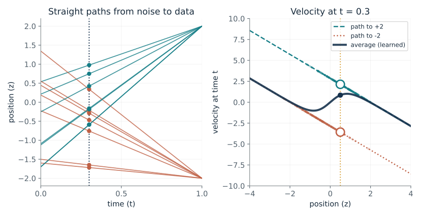
Time (t): 0.3 · Data points: two targets

At t = 0.3, paths to +2 and to -2 both pass near z = 0.5 with velocities 2.14 and -3.57. 77.3% head to +2, so the learned velocity, their average, is 0.845, equal to neither path.

Learned velocity at z = 0.5: 0.845
Velocity of a path to +2: 2.14
Velocity of a path to -2: -3.57
Paths here heading to +2 (%): 77.3

Why it matters for language models

This is why flow-matching image and video models can train on simple regression targets and still learn a flow that moves noise to the whole data distribution, not to a single example.

Show the calculation

Path: z(t) = (1 - t) x0 + t x1, velocity x1 - x0 = (x1 - z)/(1 - t). At z = 0.5, t = 0.3: (2 - 0.5)/0.7 = 2.14 and (-2 - 0.5)/0.7 = -3.57. Share to +2 = 1/(1 + exp(-4 t z/(1 - t)^2)) = 0.773; learned velocity = (E[x1 | z] - z)/(1 - t) = 0.845.

The equations and symbols

$z(t)=(1-t)\,x_0+t\,x_1,\qquad u_t(z\mid x_1)=x_1-x_0=\frac{x_1-z}{1-t}$

$\mathcal L_{\mathrm{FM}}=\mathbb E\,\|f_\theta(z(t),t)-(x_1-x_0)\|^2$

x0: a starting point drawn from the noise N(0,1)
x1: a data point; here +2 or -2
t: time, from 0 (noise) to 1 (data); t = 1 is excluded
z(t): position along the straight path at time t
u: velocity: distance covered per unit time

Where the conclusion applies

One-dimensional noise N(0,1) and data that is either the single point +2 or the two points +2 and -2 with equal probability. The scatter uses 400 seeded pairs (seed 1010); the learned velocity is the exact average over all paths through a point. Probe point z = 0.5.

Check your understanding: With only one data point, +2, what is the learned velocity at z = 0.5 and t = 0.5?

Every path goes to +2, so the velocity is (2 - 0.5) / (1 - 0.5) = 3 for all of them, and the learned velocity is 3.

Book source: Chapter 10, 10.7.1 Flow Matching: Training CNFs Without Integration. Illustration C10-D07. Illustration. Book mathematical principle with explicitly defined companion toy inputs; plotted values and worked calculations are recomputed. v39 EPUB / v43 print.

08 / 08

The two parts of FID

From Chapter 10, 10.5 Evaluation Metrics: FID, IS, and Precision-Recall

FID compares generated and real features with two Gaussians. What does each part of the score punish?

The first term is the squared distance between the two average feature vectors. The second compares the two covariance shapes and is 0 only when they are identical. Narrow, wide and turned clouds all leave a positive second term.

Predict first: Two clouds have the same centre and the same sizes along their long and short directions, but one is turned 45 degrees. Is FID zero?

Centre shift along feature 1: 1

03

Generated spread

Left: a real ellipse and a smaller dashed generated one shifted right. Right: stacked bars of centre gap and spread mismatch for four spreads. — **FID adds a centre-gap term and a spread-mismatch term; matching the centre alone does not make it small.**
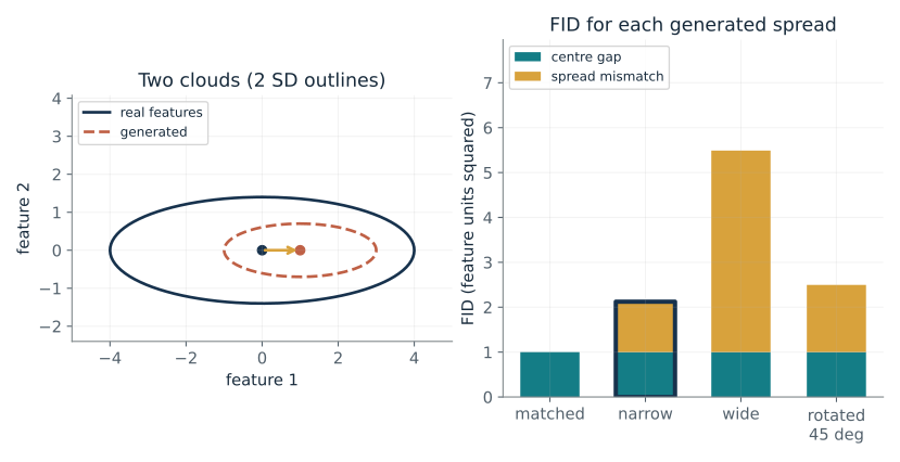
Centre shift along feature 1: 1 · Generated spread: narrow

FID adds the squared gap between centres, 1, to a term that compares the shapes. The generated cloud is narrow, which adds a spread term of 1.12. Total FID 2.12.

Centre-gap term: 1
Spread-mismatch term: 1.12
FID: 2.12

Why it matters for language models

FID is a standard image-generation benchmark. Knowing it has two parts explains why a model can have a poor FID from blurry, too-narrow outputs even when its average image is right.

Show the calculation

Centre gap squared = 1^2 = 1. Spread term = trace(S_real + S_gen - 2 (S_real S_gen)^(1/2)) = 1.12 (for scaled clouds this is (sum of variances) x (1 - scale)^2). FID = 1 + 1.12 = 2.12.

The equations and symbols

$\mathrm{FID}=\|\mu_r-\mu_g\|^2+\mathrm{tr}\left(\Sigma_r+\Sigma_g-2(\Sigma_r\Sigma_g)^{1/2}\right)$

mu_r, mu_g: average feature vector of real and generated data
Sigma_r, Sigma_g: covariance matrices: spread and orientation of each cloud
tr: trace: the sum of diagonal entries
shift: how far the generated centre is moved along feature 1

Where the conclusion applies

Two-dimensional toy features, not Inception features. Real cloud: centre (0,0), SDs 2 and 0.7 along the axes. Generated clouds are shifted along feature 1 and have the real shape, a quarter of the variance, four times the variance, or the real shape turned 45 degrees.

Check your understanding: A generated cloud has the real shape but only a quarter of the variance (half the SD). Which term is nonzero?

Only the spread term: with scale 0.5 it is (4 + 0.49) x (1 - 0.5)^2 = 1.12, while the centre gap is 0 if the centres agree.

Book source: Chapter 10, 10.5 Evaluation Metrics: FID, IS, and Precision-Recall. Illustration C10-D08. Identity. Book mathematical principle with explicitly defined companion toy inputs; plotted values and worked calculations are recomputed. v39 EPUB / v43 print.

Hidden variables make visible variation

A lower bound and its posterior gap

Separation and dropped modes

Stretching changes density, not mass

The best discriminator and the GAN value

More samples tighten the bound

Straight paths and the velocity a network learns

The two parts of FID

Bring the idea to a question of your own