Chapter 11 · Diffusion, Score, and Transport-Based Generation

Request the observed measurement, noise or blur model, available conditioning and the intended interpretation. Use a toy posterior with multiple compatible originals to explain uncertainty; return compatible alternatives and identify which details are supported by the observation versus supplied by a prior. For numeric diffusion calculations request alpha bar, the clean-data distribution and noise variance. Distinguish conditional score given a clean original from the marginal score. Explain supplied guidance settings through a clearly labeled toy score blend; consult product documentation before describing unsupplied current settings.

Try asking the chapter skill

“Why can a restored image contain convincing details that were never recorded?”

Use mathllms-ch11-diffusion with the companion's AI skill package. The illustrations below also work on their own.

01 / 08

Add a controlled amount of noise

From Chapter 11, 11.1.1 The Gaussian Perturbation Kernel

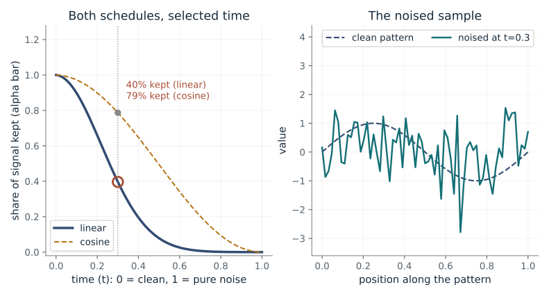
A diffusion model destroys a clean pattern step by step. How much of the original is left at a given time, and does the schedule matter?

The signal and noise weights are the square roots of the variance shares kept and removed, so they always add up to one in variance. Two schedules reach the same amount of noise at different times. The ratio of the two variance shares is the signal-to-noise ratio.

Predict first: Halfway through (t = 0.5), which schedule has thrown away more of the signal: linear or cosine?

Time (t): 0.3

00.8

Schedule

The schedule decides how fast the signal fades: at the same time the linear schedule has kept far less than the cosine one.
Time (t): 0.3 · Schedule: linear

At t=0.3 the linear schedule keeps 40% of the signal variance, the cosine one keeps 79%. The noised pattern is the clean pattern shrunk by the signal weight plus the same random draw scaled by the noise weight.

Share of signal kept (alpha bar): 0.396
Weight on the signal: 0.63
Weight on the noise: 0.777
Signal-to-noise ratio: 0.657

Why it matters for language models

Image and audio generators are trained to undo exactly this corruption. The schedule sets how much training effort goes to lightly noised versus nearly pure-noise examples.

Show the calculation

At position 0.25 the clean value is sin(pi/2) = 1 and the fixed random draw is -0.0238. Noised value = sqrt(0.396) x 1 + sqrt(0.604) x -0.0238 = 0.611. Signal-to-noise = kept / removed = 0.396 / 0.604 = 0.657. This is a ratio of variance fractions, not of the two weights. It equals the data-level ratio only when the clean data have unit variance.

The equations and symbols

$X_t=\sqrt{\bar\alpha_t}X_0+\sqrt{1-\bar\alpha_t}E$

$\mathrm{SNR}_t=\bar\alpha_t/(1-\bar\alpha_t)$

t: normalized time, 0 = clean and 1 = fully noised
alpha bar: share of the original signal variance still present at time t
X0: the clean pattern
E: random noise with unit variance
SNR: signal kept divided by noise added, as variance fractions

Where the conclusion applies

Schedules follow book 11.1.2 with T=1000 and normalized time t=n/T. Linear: beta_s rises linearly from 1e-4 to 0.02 and alpha bar_n = prod(1-beta_s), interpolated between integer steps. Cosine: alpha bar_t = f(t)/f(0) with f(t) = cos^2(((t+s)/(1+s)) pi/2) and offset s=0.008. The pattern is a fixed sine wave and the noise uses seed 1101. At t=0 nothing has been removed, so the signal-to-noise ratio is undefined (infinite).

Check your understanding: If the clean data have variance 4 and alpha bar = 0.5, what is the actual signal-to-noise ratio?

Signal variance is 0.5 x 4 = 2 and noise variance is 0.5, so the ratio is 4. The unit-variance formula alpha bar / (1 - alpha bar) would give 1.

Book source: Chapter 11, 11.1.1 The Gaussian Perturbation Kernel. Illustration C11-D01. Illustration. Book equation with companion toy inputs stated in the assumptions; every plotted value is recomputed. v39 EPUB / v43 print.

02 / 08

Read a probability landscape

From Chapter 11, 11.1.3 The Marginal Score

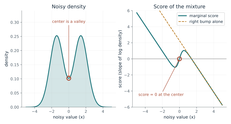
A score points uphill on the log of a density. Where does it vanish, and does a zero mean a peak?

Each bump pulls toward its own center, and the marginal score weights those pulls by how likely each bump is at x. Noise moves the centers inward and widens the bumps until they merge. At the middle the pulls cancel, which gives zero in both cases.

Predict first: With two clear bumps the center is a valley. If only 10% of the signal is kept, does the valley stay or fill in, and what happens to the score at the center?

Signal kept (alpha bar): 0.5

0.10.9

Bump offset before noise

Left: noisy two-bump density with the center marked as a valley. Right: its score crossing zero at the center, and one bump alone for comparison. — **The score is zero at the symmetric center whether it is a valley or a peak, so a zero score does not identify the shape.**
Signal kept (alpha bar): 0.5 · Bump offset before noise: 2

The score is exactly 0 at x=0 whether the center is a peak or a valley, and here the center is a valley between two bumps. Zero score marks a flat spot; it does not say whether it is a peak or a valley.

Noisy bump variance: 0.625
Right-bump share at x=1: 0.989
Marginal score at x=1: 0.614
Score at the center x=0: 0

Why it matters for language models

A diffusion network is trained to output this score. Knowing it is a share-weighted average of per-bump scores explains why samples drift toward whichever bump is currently more likely.

Show the calculation

Each original bump has variance 0.25, so the noisy variance is 0.5 x 0.25 + (1 - 0.5) = 0.625. At x=1 the right bump has share 0.989 and the left 0.0107. Their own scores are 0.663 and -3.86. Marginal score = 0.0107 x -3.86 + 0.989 x 0.663 = 0.614. This is not the score given one known clean sample, and averaging the two component scores without the shares would be wrong.

The equations and symbols

$s_t(x)=\partial_x\log p_t(x)=\sum_j r_j(x)\frac{-(x-\mu_{j,t})}{v_t}$

$\mu_{j,t}=\sqrt{\bar\alpha_t}\mu_j,\quad v_t=0.25\bar\alpha_t+1-\bar\alpha_t$

s: score: slope of the log density, pointing toward more likely values
r_j(x): share of the density at x that belongs to bump j
mu_j: bump centers before noise, at minus and plus the offset
v_t: common variance of each bump after noising
alpha bar: share of the signal still present

Where the conclusion applies

Two equally weighted Gaussian bumps with variance 0.25 before noise, centered at minus and plus the offset. Noising shrinks the centers by sqrt(alpha bar) and widens each bump to variance 0.25 alpha bar + 1 - alpha bar. Shares are computed in log space. This marginal score is different from the score given one known clean sample.

Check your understanding: For any equal mixture of two bumps placed symmetrically, what is the marginal score at x = 0?

Zero, because the two shares are equal and the two component scores cancel. Zero alone does not say whether the center is a maximum or a minimum.

Book source: Chapter 11, 11.1.3 The Marginal Score. Illustration C11-D02. Illustration. Book equation with companion toy inputs stated in the assumptions; every plotted value is recomputed. v39 EPUB / v43 print.

03 / 08

Two return journeys

From Chapter 11, 11.7.1 The Probability-Flow ODE

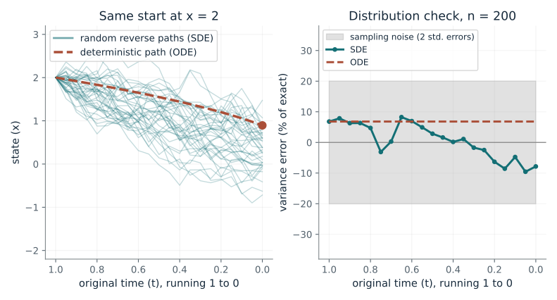
A random reverse path and a deterministic one start from the same noisy value. Do they end at the same place, and do their distributions agree?

The reverse SDE adds new randomness while the probability-flow ODE evolves deterministically, and their drifts differ by a factor of two. Correctly started, both match the exact distribution at every time. That statement is about distributions, not about individual paired samples.

Predict first: With 200 samples the variance curves wander several percent from the exact value. About how many samples bring the error under 3%?

Number of samples (n): 200

5030000

Clean data variance (v0)

Left: 40 random reverse paths fan out from x=2 while one dashed ODE path ends elsewhere. Right: variance errors inside a grey sampling band. — **The SDE and ODE end at different points from the same start, yet both reproduce the exact variance up to sampling noise.**
Number of samples (n): 200 · Clean data variance (v0): 0.25

Every path on the left starts at x = 2. The ODE ends at 0.894; the SDE paths end spread out (std. dev. 0.461). On the right both variance curves stay near the exact value, within sampling noise, so the two methods give the same distribution.

Exact variance at t=0: 0.25
SDE sample variance at t=0: 0.23
ODE sample variance at t=0: 0.267
Spread of the 40 SDE end points: 0.461

Why it matters for language models

Fast samplers for diffusion models choose between a random and a deterministic way of undoing noise. Both come from the same learned score, so the choice does not change the distribution of samples. The ODE is deterministic and invertible, which allows fewer steps; the SDE adds fresh noise that can correct earlier errors.

Show the calculation

Forward process: f = 0, g = 1, so the variance at time t is 0.25 + t and the score is s = -x / (0.25 + t). The reverse SDE has drift coefficient -s and the ODE has -s/2, both multiplying dt. Original time falls, so dt is negative and a positive coefficient pulls x toward 0. One exact backward step of h = 0.05 from variance v = 1.25: the SDE multiplies x by 0.96 and adds noise of variance 0.048; the ODE multiplies by sqrt(0.96) = 0.98. Left plot uses 40 SDE paths; right plot uses 200 samples.

The equations and symbols

$dX=(f-g^2s_t)\,dt+g\,d\bar W_t,\qquad dX=(f-\tfrac12g^2s_t)\,dt$

$f=0,\quad g=1,\quad s_t(x)=-x/(v_0+t),\quad t:1\to0$

SDE: reverse process that adds fresh randomness at every step
ODE: reverse process with no randomness (probability flow)
s_t: exact score of the noised density at time t
v0: variance of the clean data; at time t it is v0 + t
n: number of samples used to estimate each variance

Where the conclusion applies

Exact terminal law, exact Gaussian scores and exact backward updates for both processes, 20 backward intervals. Seed 1103 draws the n shared terminal values and the independent SDE noise; seed 1105 draws the 40 paths on the left. The ODE is probability flow, not the SDE without its noise; the factor one-half is necessary. The grey band is plus or minus two standard errors of a Gaussian sample variance, 2 sqrt(2/(n-1)).

Check your understanding: For v0 = 1, t = 1 and x = 2, what are the reverse SDE and ODE drift coefficients of dt?

The score is -2/(1+1) = -1. With f = 0 and g = 1 the SDE coefficient is 1 and the ODE coefficient is 0.5. Since dt is negative, x moves toward 0 in both cases.

Book source: Chapter 11, 11.7.1 The Probability-Flow ODE. Illustration C11-D03. Illustration. Book equation with companion toy inputs stated in the assumptions; every plotted value is recomputed. v39 EPUB / v43 print.

04 / 08

Conditioning changes direction

From Chapter 11, 11.7.3 Classifier and Classifier-Free Guidance

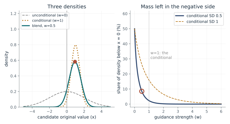
What does turning up the guidance strength do to the spread of answers in this toy?

The score blend changes the slope of the log density. Here the result is again a Gaussian whose precision is a weighted sum of the two precisions. Larger w therefore narrows it and shifts its mean; this toy tradeoff is not a general theorem about image quality.

Predict first: Will w = 2 reproduce the conditional density, or go beyond it?

Guidance strength (w): 0.5

Conditional std. dev.

Guidance above 1 does not copy the conditional: it narrows the density further and moves its center slightly past the condition.
Guidance strength (w): 0.5 · Conditional std. dev.: 0.5

At w=0.5 the blended density has mean 0.941 and std. dev. 0.686; the conditional alone has mean 1 and 0.5. Raising w narrows it further and leaves less density on the negative side.

Blended mean: 0.941
Blended standard deviation: 0.686
Share of density below 0: 8.5%
Score at x=0: 2

Why it matters for language models

Classifier-free guidance in text-to-image models mixes a conditional and an unconditional prediction in this way. Higher strength follows the prompt more tightly and gives less variety.

Show the calculation

At x=0 the unconditional score is 0 and the conditional score is 1/0.5^2 = 4. The blend is 0 + 0.5 x 4 = 2. Completing the square in p0^(1-w) pc^w gives precision (1-w)/4 + w/0.5^2 = 2.12, so mean = 0.941 and std. dev. = 0.686. This is an exact density blend at one fixed time, not a claim about whole guided reverse processes.

The equations and symbols

$\tilde s=s_\varnothing+w(s_c-s_\varnothing)$

$\tilde s=\partial_x\log\left(p_\varnothing^{1-w}p_c^w\right)$

w: guidance strength: 0 unconditional, 1 conditional, above 1 extrapolated
s_0: score with no condition, from N(0, 4)
s_c: score given the condition, from N(1, width^2)
width: standard deviation of the conditional density

Where the conclusion applies

Both Gaussian densities are positive and the combined precision (1-w)/4 + w/width^2 stays positive for every preset. The blend of scores is not a probability mixture of the densities, and nothing here claims anything about a whole guided reverse process.

Check your understanding: If two different originals produce the same blurred observation, does strong guidance prove which one occurred?

No. Conditioning can favor an alternative the prior likes, but it cannot create evidence that separates originals the measurement does not distinguish.

Book source: Chapter 11, 11.7.3 Classifier and Classifier-Free Guidance. Illustration C11-D04. Illustration. Book equation with companion toy inputs stated in the assumptions; every plotted value is recomputed. v39 EPUB / v43 print.

05 / 08

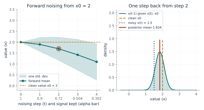
A four-step noising trace by hand

From Chapter 11, 11.13.1 DDPM Forward and Reverse Process: Numerical Trace

Starting from the clean value 2, what do four noising steps do, and where does one denoising step land?

The left plot shows the forward marginal: the mean shrinks by the square root of the kept share while the spread grows. The right plot applies Bayes rule for one step back when the clean value is known, giving a Gaussian with the weights shown in the calculation.

Predict first: With x0 = 2 and x_t = 1.5, the posterior mean at step 2 is close to x0. Moving to step 3, does it move toward x0 or toward x_t?

Noisy value (x_t): 1.5

03.5

Step (t)

Left: mean and spread of the noised value over four steps with the selected step circled. Right: posterior density with x0, x_t and its mean marked. — **Each step back is a weighted blend of the clean value and the noisy value, and the weight on the noisy value grows as more noise is present.**
Noisy value (x_t): 1.5 · Step (t): 2

With x0 = 2 known and x(t) = 1.5, one step back lands near 1.834, a blend of the clean value and the noisy one. At step 2 the clean value gets weight 0.68; later steps trust the noisy value more.

Signal kept after t steps: 0.72
Weights on x0 and x(t): 0.678 and 0.319
Posterior mean: 1.834
Posterior variance: 0.0714

Why it matters for language models

This is the arithmetic of diffusion training: the noised input comes from the forward marginal and the posterior mean is the target that a denoising network learns to approximate.

Show the calculation

abar(1) = 0.9, abar(2) = 0.72, beta(2) = 0.2. Weight on x0 = sqrt(0.9) x 0.2 / 0.28 = 0.678. Weight on x(t) = sqrt(0.8) x 0.1 / 0.28 = 0.319. Mean = 0.678 x 2 + 0.319 x 1.5 = 1.355 + 0.4792 = 1.834. Variance = 0.1 / 0.28 x 0.2 = 0.0714.

The equations and symbols

$\bar\alpha_t=\prod_{s\le t}(1-\beta_s),\quad q(x_t\mid x_0)=\mathcal N(\sqrt{\bar\alpha_t}x_0,\,1-\bar\alpha_t)$

$\tilde\mu=\frac{\sqrt{\bar\alpha_{t-1}}\beta_t}{1-\bar\alpha_t}x_0+\frac{\sqrt{\alpha_t}(1-\bar\alpha_{t-1})}{1-\bar\alpha_t}x_t$

beta_t: noise added at step t: 0.1, 0.2, 0.3, 0.4
alpha bar: running product of (1 - beta): signal variance kept
x0: clean value, here 2
x_t: noisy value at step t
mu tilde: mean of the one-step-back posterior given x0 and x_t

Where the conclusion applies

Exactly four steps with the book betas. The posterior q(x_{t-1} | x_t, x0) conditions on the known clean value, as in training; it is not a sampling step, because at generation time x0 is unknown. Defined for t = 2, 3, 4; at t = 1 it would be a point mass at x0.

Check your understanding: If x0 = 2 and x_t = 2 at step 3, is the posterior mean above or below 2?

Below, at 1.97. The two weights 0.513 and 0.472 add to 0.986, less than 1, so the mean is pulled slightly toward 0.

Book source: Chapter 11, 11.13.1 DDPM Forward and Reverse Process: Numerical Trace. Illustration C11-D05. Identity. Book worked example with its own numbers (beta 0.1, 0.2, 0.3, 0.4; x0 = 2; x_t = 1.5 at t = 3); values are recomputed. The book rounds alpha bar_4 to 0.302 (exactly 0.3024). v39 EPUB / v43 print.

06 / 08

Matching two sets of points with Sinkhorn

From Chapter 11, 11.13.2 Schrödinger Bridge Sinkhorn Iteration

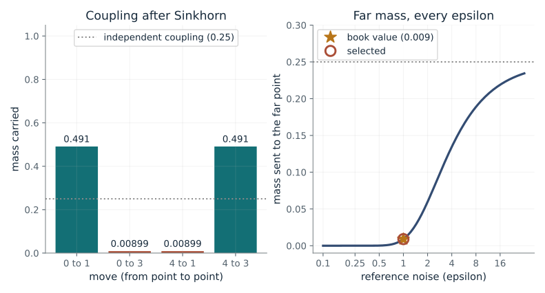
Two points must be carried to two other points. How does the amount of reference noise decide where the mass goes?

The kernel rewards pairs that Brownian motion would link easily. Sinkhorn rescales its rows and columns until each start gives away exactly 0.5 and each end receives exactly 0.5. Rescaling keeps the ratio between near and far entries, so epsilon alone sets how much mass goes far.

Predict first: If the reference noise epsilon grows from 1 to 16, does the coupling stay near the diagonal or spread out? Toward what limit?

Reference noise (epsilon): 1

0.116

Stage

Left: four bars of mass carried, two large near moves and two near-zero far moves. Right: far mass rising with epsilon toward 0.25. — **Small reference noise keeps the coupling close to the nearest points; large noise washes it out toward the independent coupling.**
Reference noise (epsilon): 1 · Stage: Sinkhorn

After Sinkhorn scaling each row carries 0.5. At epsilon 1 only 0.00899 of it goes to the far point; a small epsilon keeps the coupling near the diagonal, a large one spreads it toward the independent 0.25.

Mass sent 0 to 1 (near): 0.491
Mass sent 0 to 3 (far): 0.00899
Total mass: 1
Kernel ratio far / near: 0.0183

Why it matters for language models

Entropy-regularized transport computed by Sinkhorn is a standard way to match two sets of samples, in generative modelling and in comparing sets of embeddings; epsilon sets how sharply points are paired.

Show the calculation

K(0,1) = exp(-1 / (2 x 1)) = 0.607; K(0,3) = exp(-9 / (2 x 1)) = 0.0111. Row sum = 0.618, so phi0 = 0.5 / 0.618 = 0.81 and phi1 = 1 by symmetry. Entry (0,1) = 0.81 x 0.607 = 0.491; entry (0,3) = 0.81 x 0.0111 = 0.00899. One scaling sweep already converges here because the example is symmetric.

The equations and symbols

$K_{ij}=\exp\!\left(-\frac{|x_i-y_j|^2}{2\varepsilon}\right)$

$\pi^*_{ij}=\phi_0(i)\,K_{ij}\,\hat\phi_1(j)$

epsilon: noise level of the Brownian reference (the book uses 1)
K: kernel: how naturally Brownian motion links start i to end j
phi: scaling vectors found by Sinkhorn so that rows and columns carry the right mass
pi: coupling: mass carried from each start to each end

Where the conclusion applies

Start points 0 and 4, end points 1 and 3, equal masses 0.5, Brownian kernel exp(-d^2/(2 epsilon)). Sinkhorn alternates dividing by row sums and column sums; this symmetric example converges after one sweep, and 60 sweeps are run. The raw kernel is shown for comparison and is not a coupling.

Check your understanding: If epsilon doubles from 1 to 2, does the far mass roughly double?

No, it grows about seven times, from 0.009 to 0.060. The far/near ratio is exp(-4/epsilon) (so near/far is exp(4/epsilon)), which changes quickly when epsilon is small.

Book source: Chapter 11, 11.13.2 Schrödinger Bridge Sinkhorn Iteration. Illustration C11-D06. Identity. Book worked example (starts 0 and 4, ends 1 and 3, each with mass 0.5, epsilon = 1 gives 0.491 and 0.009); the epsilon slider is a companion extension. v39 EPUB / v43 print.

07 / 08

Langevin dynamics gets stuck or blurs

From Chapter 11, 11.3 Langevin Dynamics

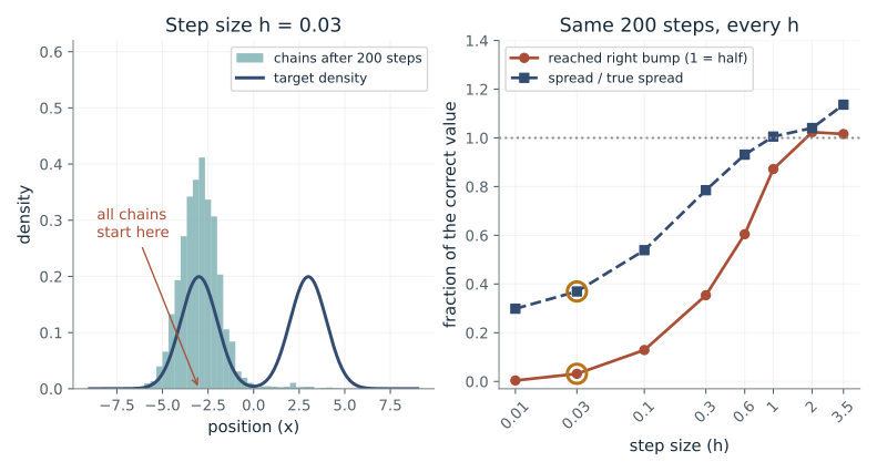
A sampler follows the score plus noise. With a fixed budget of 200 steps, how does the step size decide whether it visits both bumps?

The chain moves by a drift toward higher density plus noise. Crossing the low-density valley takes enough total time h x steps for noise to push a chain over, while too large an h makes each update inaccurate. The fixed budget of 200 steps makes the two effects visible.

Predict first: All chains start in the left bump. With the same 200 steps, does a very small step size help them reach the right bump?

Step size (h): 0.03

0.013.5

Left: histogram of sampler positions against a two-bump target, all chains stuck in the left bump. Right: mixing and spread against step size. — **Step size trades coverage against accuracy: tiny steps never cross to the other bump, large steps cross but blur the target.**
Step size (h): 0.03

1.57% of the chains are in the right bump (the target has 50%). Almost no chain crosses the valley: the steps are too small to cover enough time, so the sample is stuck in one bump.

Chains in right bump: 1.57%
Spread of samples (true 3.16): 1.17
Time covered (h x 200): 6
Step size limit near a bump: 4

Why it matters for language models

Score-based generators draw samples by following a learned score plus noise. A sampler that never leaves its starting mode gives low variety, which is a similar symptom to mode collapse in other generators, though the mechanism differs.

Show the calculation

Each step: x_new = x + (h/2) s(x) + sqrt(h) z with score s(x) = -x + 3 tanh(3x) for the bumps at -3 and +3. From x = -3 the score is about 0, so each step is mostly noise of size sqrt(0.03) = 0.173. 200 steps cover time 6. Near one bump the update is x_new = (1 - h/2) x + sqrt(h) z, which is stable only for h < 4, and in that linearized update its long-run variance is 1 / (1 - h/4) = 1.008, against 1 for a single exact bump. This is a per-bump value; the measured spread also includes the distance between bumps.

The equations and symbols

$d X_t=\tfrac12\nabla\log p(X_t)\,dt+dW_t$

$x_{k+1}=x_k+\tfrac h2\,s(x_k)+\sqrt h\,z_k,\quad s(x)=-x+3\tanh(3x)$

h: step size of the discrete sampler
s(x): score of the target density, here two bumps at minus 3 and plus 3
z: fresh standard normal noise at each step
x: sampler position

Where the conclusion applies

Target: equal mixture of N(-3,1) and N(3,1), true spread sqrt(10) = 3.16. 4000 chains all start at x = -3 and take 200 Euler steps (seed 1107). Around one bump the update is stable only for h < 4. Large steps carry discretization bias; no accept/reject correction is used.

Check your understanding: Would 800 steps at h = 0.03 cross as well as 200 steps at h = 0.1?

About the same: the time covered is 24 against 20, and what matters for crossing is time, not step count. Only about 6% of chains cross at h = 0.1 here.

Book source: Chapter 11, 11.3 Langevin Dynamics. Illustration C11-D07. Illustration. Book Langevin SDE and its stationarity (Proposition 11.1); the two-bump target, 200 steps and seeded chains are companion toys. Nothing is tuned. v39 EPUB / v43 print.

08 / 08

Unmasking a hidden token

From Chapter 11, 11.14.1 The Absorbing-State Transition and Its Closed-Form Posterior

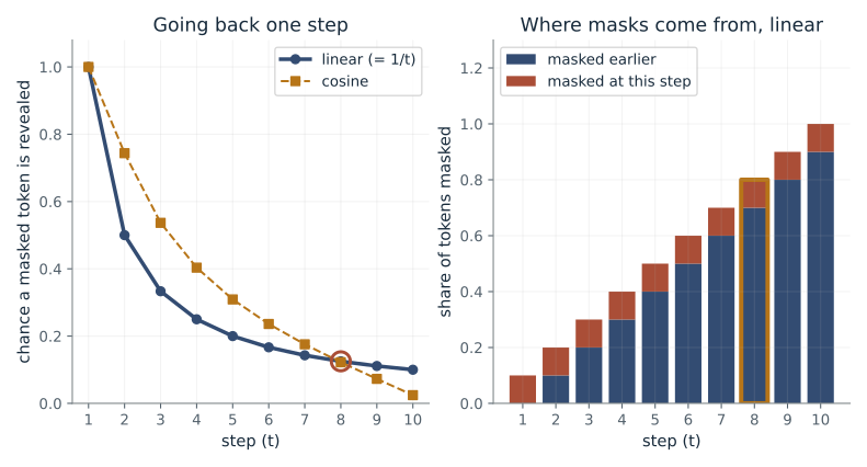
In masked diffusion for text, a token is replaced by a mask and never un-masked going forward. Going backward, what is the chance a masked token is revealed at step t?

A masked token was either masked at this very step or already masked before it. Dividing the first probability by their sum gives the reveal chance. Visible tokens are never touched in the reverse step, so only masked positions need a prediction.

Predict first: Under the linear schedule, a token masked at step 8 is revealed going back with what chance, compared with one masked at step 2?

Step (t): 8

Schedule

Left: chance a masked token is revealed falling with step for linear and cosine. Right: stacked bars of old and new masks at each step. — **Given a mask at step t, the chance it was just applied is the new-mask share of all masks, which is 1/t for the linear schedule.**
Step (t): 8 · Schedule: linear

A token that is masked at step 8 was masked just now with chance 0.125, so going back it is revealed with that chance, otherwise it stays masked. Under the linear schedule this chance is exactly 1/t, high early and low late.

Masked at step t: 0.8
Masked earlier: 0.7
Newly masked at this step: 0.1
Chance revealed going back: 0.125

Why it matters for language models

Masked diffusion language models are trained by hiding tokens and predicting them. This chance sets how many tokens are revealed per denoising step and the weight of each step in the training loss.

Show the calculation

Linear schedule with T = 10: abar(7) = 0.3, abar(8) = 0.2. Newly masked = 0.3 - 0.2 = 0.1. Masked earlier = 1 - 0.3 = 0.7. Total masked = 0.1 + 0.7 = 0.8. Chance revealed = 0.1 / 0.8 = 0.125.

The equations and symbols

$q(x_{t-1}=x_0\mid x_t=m,x_0)=\frac{\bar\alpha_{t-1}(1-\alpha_t)}{1-\bar\alpha_t}$

$\bar\alpha_{t}=1-t/T\ \Rightarrow\ \text{chance}=1/t$

m: the mask symbol
alpha_t: chance a visible token survives step t
alpha bar: chance a token is still visible after t steps
T: number of steps, 10 here

Where the conclusion applies

Linear schedule alpha bar_t = 1 - t/T; cosine schedule alpha bar_t = cos^2(pi t / (2T)). At t = T every token is masked. A token masked at step t was either masked earlier or masked exactly at step t; these two events split the total probability 1 - alpha bar_t.

Check your understanding: With the linear schedule and T = 20, what is the chance a token masked at step 4 is revealed going back?

0.25, which is 1/4. For the linear schedule the chance is 1/t whatever T is.

Book source: Chapter 11, 11.14.1 The Absorbing-State Transition and Its Closed-Form Posterior. Illustration C11-D08. Identity. Book Proposition 11.2 (absorbing-state posterior); T = 10 and the linear and cosine survival schedules are companion toys, with the book linear and cosine forms. v39 EPUB / v43 print.

Bring the idea to a question of your own

The chapter skill can adapt the calculations to your inputs. It should identify the assumptions, explain what the result supports, and show what still needs evidence.