Chapter 12 · Continuous-Depth and Implicit Models

01 / 08

Steps approximate continuous decay

From Chapter 12, 12.1.1 The Euler Correspondence

A quantity decays smoothly. When does a computer that follows it in steps draw the wrong picture?

Euler replaces the smooth curve by a straight tangent step. Each step multiplies the state by 1 - ah. That factor is positive and small for small steps, negative for steps past ah = 1, and larger than 1 in size past ah = 2.

Predict first: If the step times the rate (ah) is 2.4, do both the exact solution and the Euler steps decay?

Euler step size (h): 1.5

0.253

Decay rate (a)

Left: smooth exact decay and zigzag Euler steps. Right: the factor per step against ah, with the limit at 2 and the chosen point circled. — **Euler follows the decay only while ah is below 2, and it keeps the smooth shape only while ah is below 1.**
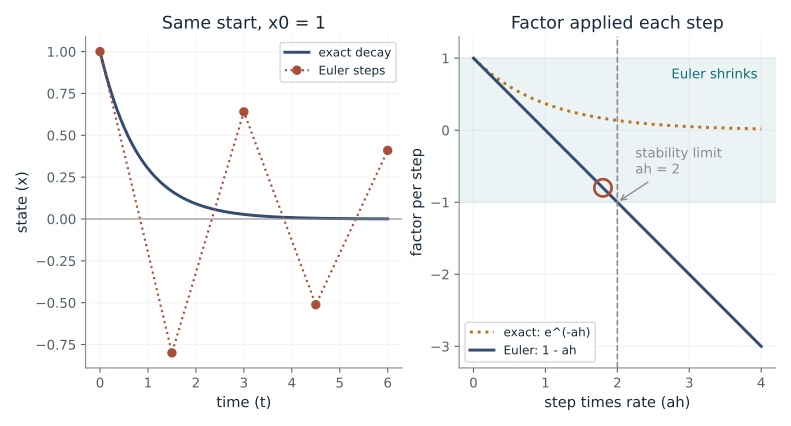
Euler step size (h): 1.5 · Decay rate (a): 1.2

The exact answer always decays smoothly. With ah = 1.8, Euler multiplies by -0.8 each step, so it flips sign every step but still shrinks. Euler is trustworthy only while ah stays below 2, and even then it gets the shape right only when ah is below 1.

Euler factor per step (1 - ah): -0.8
Exact factor per step (e^(-ah)): 0.165
Euler shrinks?: yes
Error at time 6: 0.409

Why it matters for language models

A residual layer rescaled as x + (1/L) f(x) is one Euler step of size 1/L (the book's Euler correspondence, which does not hold for every standard ResNet), so a layer that is too strong for its dynamics can flip and amplify the signal instead of shrinking it.

Show the calculation

First step: x1 = x0 + h(-a x0) = 1 - 1.5 x 1.2 x 1 = -0.8. After 4 steps Euler gives (-0.8)^4 = 0.41 at time 6; the exact value is e^(-1.2 x 6) = 0.000747.

The equations and symbols

$\dot x=-ax,\quad x(t)=e^{-at}x_0,\qquad x_n=(1-ah)^nx_0$

x: the state, starting at 1
a: decay rate: how fast the exact answer shrinks
h: step size of the solver, in time units
ah: step times rate, a pure number
n: number of steps taken

Where the conclusion applies

Fixed time horizon 6 and positive rates. Explicit Euler shrinks only when 0 < ah < 2, and it keeps the smooth shape of the exact answer only when ah < 1. The step sizes shown divide 6 evenly.

Check your understanding: For a = 2 and h = 0.75, what is the Euler factor, and does Euler shrink?

The factor is 1 - 1.5 = -0.5. Its size is below one, so it shrinks, but it alternates sign, unlike the exact positive decay.

Book source: Chapter 12, 12.1.1 The Euler Correspondence. Illustration C12-D01. Illustration. Book equation with companion toy inputs stated in the assumptions; every plotted value is recomputed. v39 EPUB / v43 print.

02 / 08

Updating can fail to settle

From Chapter 12, 12.4.2 Existence via Banach Fixed-Point Theorem

If an update rule has a resting value, will repeating the rule actually arrive there?

Solving an equation and reaching its solution by repetition are different tasks. The error recurrence shows why: each update multiplies the distance from the fixed point by theta. A distance multiplied by something above 1 in size can only grow.

Predict first: For theta = -1.2, can a resting value exist even while the iteration flips sign and grows?

Feedback multiplier (theta): 1.2

-1.21.2

Constant input (x)

Left: cobweb path climbing away from the fixed point for theta 1.2. Right: iterates growing while the fixed point stays at -5. — **A fixed point can exist and still never be reached: the repeated update settles from the start only when |theta| is below 1.**
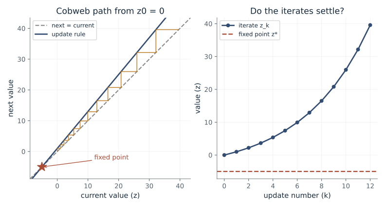
Feedback multiplier (theta): 1.2 · Constant input (x): 1

The fixed point -5 exists, yet the iterates move away from it, because |theta| is above 1. Having a solution and reaching it by repeated updates are two separate questions.

Fixed point (z*): -5
Size of multiplier |theta|: 1.2
Iteration settles?: no
Distance from z* after 12 updates: 44.6

Why it matters for language models

A deep equilibrium model repeats one layer until its output stops changing; whether it stops depends on the layer's multiplier staying below 1, not on a solution merely existing.

Show the calculation

First update: z1 = 1.2 x 0 + 1 = 1. Second: z2 = 1.2 x 1 + 1 = 2.2. Fixed point: z* = x / (1 - theta) = 1 / (1 - (1.2)) = -5. The error obeys z_k - z* = theta^k (z0 - z*), which shrinks only when |theta| < 1.

The equations and symbols

$z_{k+1}=\theta z_k+x,\qquad z^*=x/(1-\theta)\quad(\theta\ne1)$

$z_k-z^*=\theta^k(z_0-z^*)$

theta: feedback multiplier applied at each update
x: constant input added at each update
z_k: value after k updates, starting at z0 = 0
z*: fixed point: the value the rule leaves unchanged

Where the conclusion applies

A fixed point exists for theta other than 1 even outside contraction. At theta = 1 with x = 1 none exists; at theta = 1 with x = 0 every value is fixed. Starting from z0 = 0, convergence requires |theta| < 1. Twelve updates are shown.

Check your understanding: What happens when theta = 1 and x = 0, compared with theta = 1 and x = 1?

With x = 0 every value is fixed, so the start never moves. With x = 1 no fixed point exists and the value grows by one each round.

Book source: Chapter 12, 12.4.2 Existence via Banach Fixed-Point Theorem. Illustration C12-D02. Illustration. Book equation with companion toy inputs stated in the assumptions; every plotted value is recomputed. v39 EPUB / v43 print.

03 / 08

An equilibrium can be sensitive

From Chapter 12, 12.4.4 Implicit Differentiation for DEQs

How well does a slope predict how much a resting value moves when a setting changes?

The denominator 1 - theta shrinks as theta approaches 1, so the resting value changes more and more per step in theta. For this update, the slope is x/(1-theta)^2, which has the sign of x. A real change also moves the denominator, so the straight-line estimate is only approximate.

Predict first: As theta approaches one, does the slope of the equilibrium necessarily become positive?

Feedback multiplier (theta): 0.8

0.20.95

Constant input (x)

Left: the equilibrium curve rising sharply toward theta 1 with a tangent line. Right: two bars, slope estimate 0.25 and actual change 0.263. — **The slope x/(1-theta)^2 predicts how the equilibrium moves, but it grows without limit near theta = 1 and understates the size of a finite change.**
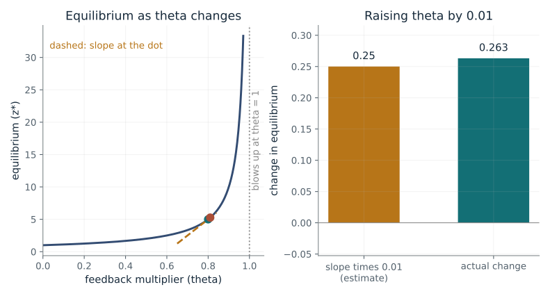
Feedback multiplier (theta): 0.8 · Constant input (x): 1

Raising theta by 0.01 moves the equilibrium from 5 to 5.26. The slope predicted 0.25, so the actual change is 5% larger, and the gap widens as theta nears 1 because the denominator keeps shrinking. The sign of the slope follows the sign of x.

Equilibrium (z*): 5
Slope dz*/dtheta: 25
Slope estimate of the change: 0.25
Actual change: 0.263

Why it matters for language models

Training a deep equilibrium layer needs the gradient of its fixed point with respect to its weights, and that gradient contains the factor 1/(1-theta): layers close to the edge of stability give very large gradients.

Show the calculation

z* = x / (1 - theta) = 1 / 0.2 = 5. Slope = x / (1 - theta)^2 = 1 / 0.2^2 = 25. Estimate = slope x 0.01 = 0.25. New equilibrium at theta + 0.01 = 0.81: 1 / 0.19 = 5.263, so the actual change is 5.263 - 5 = 0.263.

The equations and symbols

$\frac{\partial z^*}{\partial\theta}=(I-J_f)^{-1}\frac{\partial f}{\partial\theta},\qquad J_f=\left.\frac{\partial f}{\partial z}\right|_{z^*}$

$\frac{\partial z^*}{\partial\theta}=\frac{x}{(1-\theta)^2}$

$\Delta z^*\approx\frac{x}{(1-\theta)^2}\Delta\theta$

theta: feedback multiplier
x: constant input
z*: equilibrium, x / (1 - theta)
delta theta: the change made to theta, fixed at 0.01
J_f: how the update map changes with z at the equilibrium (here just theta)

Where the conclusion applies

The change delta theta = 0.01 never reaches theta = 1. Exact equilibria are compared, not unconverged iterates. Inputs include negative and zero values to show that the sign follows x and that x = 0 gives zero sensitivity. The general formula needs I - J_f to be invertible; convergence of the iteration is a separate condition.

Check your understanding: For theta = 0.5 and x = -2, what is the slope of the equilibrium?

It is -2/(0.5)^2 = -8, so increasing theta slightly lowers the equilibrium. The size grows near one; the sign stays negative.

Book source: Chapter 12, 12.4.4 Implicit Differentiation for DEQs. Illustration C12-D03. Illustration. Book equation with companion toy inputs stated in the assumptions; every plotted value is recomputed. v39 EPUB / v43 print.

04 / 08

Numerics can distort conserved energy

From Chapter 12, 12.9.3 Symplectic Integrators

What does the Stormer-Verlet update keep, and what does Euler spoil?

The exact orbit stays on a circle of fixed energy. Euler multiplies the energy by 1 + h^2 at each step, so the orbit spirals outward. Verlet's energy only wobbles, but its frequency is 2 asin(h/2)/h instead of 1, so the phase slowly drifts.

Predict first: If a simulated orbit keeps its energy, is its timing also right?

Time step (h): 0.5

0.11.25

Time horizon

Left: a nearly circular Verlet orbit with Euler spiralling out of view. Right: Euler energy rising on a log scale, Verlet staying near 1. — **Euler adds energy at every step while Verlet keeps it bounded, but Verlet still runs at a slightly wrong frequency, so energy and timing are separate checks.**
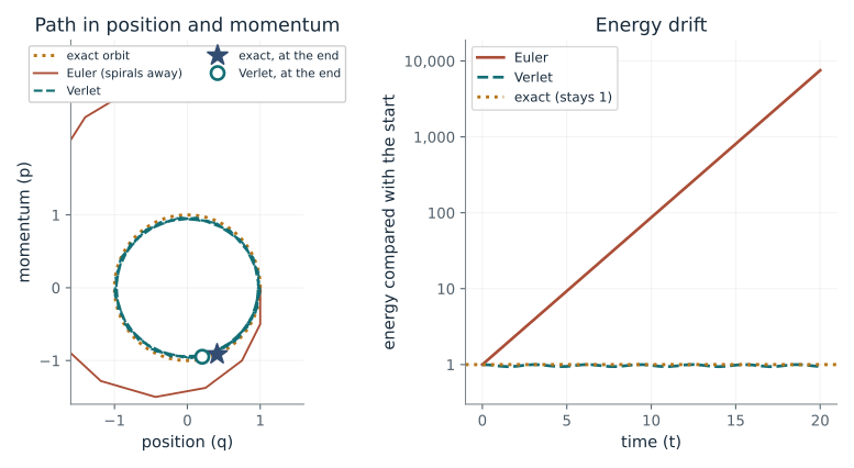
Time step (h): 0.5 · Time horizon: 20

Euler pumps energy in every step and the orbit spirals outward, ending at 7,520 times the starting energy. Verlet keeps its energy between 0.469 and 0.5, yet its timing is estimated to end 0.214 radians off, so steady energy does not mean correct timing.

Euler energy at the end (start 0.5): 3,760
Verlet energy range: 0.469 to 0.5
Verlet phase drift, formula estimate (radians): 0.214
Verlet frequency above exact (exact: 0): 0.0107

Why it matters for language models

Hamiltonian neural networks (book 12.9) are integrated with symplectic updates for this reason: a long rollout stays on the right energy surface, although its timing may still drift.

Show the calculation

Verlet first step with q0 = 1, p0 = 0: half kick gives p = -0.5/2 = -0.25, then q1 = 1 - 0.5^2/2 = 0.875, then p1 = -0.469. Euler multiplies energy by 1 + h^2 = 1.25 per step, so after 40 steps H = 0.5 x 1.25^40 = 3,760. Verlet frequency 2 asin(h/2) / h exceeds the exact value 1 by 0.0107, so over time 20 the phase drift estimate is 0.0107 x 20 = 0.214 radians.

The equations and symbols

$H=(q^2+p^2)/2,\quad \dot q=p,\quad \dot p=-q$

$p_{n+1/2}=p_n-hq_n/2,\quad q_{n+1}=q_n+hp_{n+1/2},\quad p_{n+1}=p_{n+1/2}-hq_{n+1}/2$

q: position of the oscillator
p: momentum of the oscillator
H: energy, starting at 0.5 for q = 1, p = 0
h: time step

Where the conclusion applies

Explicit Euler is compared with the book's half-kick, full-drift, half-kick Stormer-Verlet update. All steps shown are below 2, the stable range. Bounded energy wobble is not exact conservation. Horizon steps divide 10 and 20 evenly.

Check your understanding: Starting with H = 0.5, what energy does Euler have after two steps of h = 0.5?

Each step multiplies the energy by 1 + 0.25 = 1.25, so after two steps it is 0.5 x 1.25^2 = 0.78125.

Book source: Chapter 12, 12.9.3 Symplectic Integrators. Illustration C12-D04. Illustration. Book equation with companion toy inputs stated in the assumptions; every plotted value is recomputed. v39 EPUB / v43 print.

05 / 08

One-dimensional flows cannot cross

From Chapter 12, 12.2.1 Continuous Flows and Diffeomorphisms

Can a continuous-depth layer on a single number swap two inputs, and what does an extra coordinate change?

If two paths on a line met, they would have to start from the same point at that moment, and a flow with unique solutions never allows it. So the order along the line is frozen. A second coordinate gives room to pass: the points can sit at different heights while their x positions swap.

Predict first: Can a flow on one number move A to where B started and B to where A started? What changes if one coordinate is added?

Flow time (t): 1

01

Added coordinate

Left: points A and B approaching each other on a line, hollow marks showing swapped targets. Right: x gap of B minus A against time for both cases. — **In one dimension trajectories cannot cross, so no flow can swap two points; one extra coordinate lets them go around each other.**
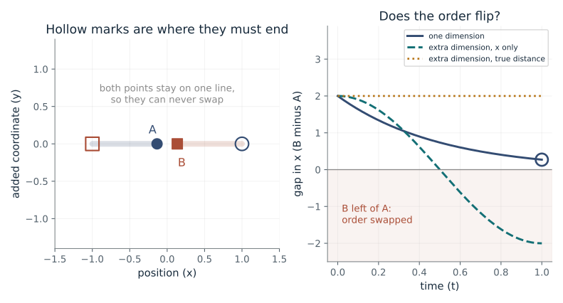
Flow time (t): 1 · Added coordinate: none

In one dimension the two paths cannot cross, so the gap 0.271 stays above zero at every time. No smooth flow can swap A and B, whatever the vector field, because swapping would force the paths to meet.

Position of A (starts at -1): x = -0.135
Position of B (starts at +1): x = 0.135
Gap in x (B minus A): 0.271
Order of A and B along x: kept (A still left of B)

Why it matters for language models

A continuous-depth layer is a smooth, invertible map, so a narrow one cannot reverse the order of values, such as sending x to -x in one feature. Giving the hidden state extra width, as augmented Neural ODEs do, removes that limit.

Show the calculation

Flow dx/dt = -2x gives x(t) = x0 e^(-2t). At t = 1: A = -e^(-2 x 1) = -0.135, B = 0.135, gap = 2 e^(-2 x 1) = 0.271.

The equations and symbols

$\dot x=f(x,t):\quad x_B(0)>x_A(0)\ \Rightarrow\ x_B(t)>x_A(t)\ \text{for all }t$

$\dot x=-\pi y,\ \dot y=\pi x\ \Rightarrow\ (x,y)(t)=x_0(\cos\pi t,\ \sin\pi t)$

A, B: two starting points, A at -1 and B at +1
t: flow time, from 0 to 1
y: the added coordinate, which starts at 0
gap: x position of B minus x position of A

Where the conclusion applies

One-dimensional flows with unique solutions cannot cross, so they keep the order of the points; dx/dt = -2x is one example of this. With one added coordinate the state is (x, y) starting at (x0, 0), and the rotation flow swaps the two points by time 1 along non-touching paths.

Check your understanding: Could a two-dimensional flow swap A and B if both were forced to stay on the x axis?

No. Staying on the axis makes it a one-dimensional flow again, and order cannot change. The freedom comes from leaving the line.

Book source: Chapter 12, 12.2.1 Continuous Flows and Diffeomorphisms. Illustration C12-D05. Illustration. Book Theorem 12.3 and Figure 12.1 (augmentation, Definition 12.2). The flow dx/dt = -2x is the book's picture example; the half-turn rotation is a companion construction. v39 EPUB / v43 print.

06 / 08

Euler against RK4: order of a solver

From Chapter 12, 12.1.3 Numerical ODE Solvers as Architecture Choices

When a solver's step is halved, how fast does its error fall, and is a fancier method worth four evaluations per step?

Euler uses one slope per step. RK4 samples the slope at the start, twice in the middle and at the end, and averages them with weights 1, 2, 2, 1. That cancels error terms through h^4, so halving h divides the error by about 2^4 = 16 instead of 2.

Predict first: If you halve the step size, by what factor does the error of each method fall?

Number of steps: 4

132

Horizontal axis of the error plot

Left: exact decay with Euler and RK4 step points. Right: error against network evaluations on log scales, RK4 far below Euler. — **Euler is first order (error roughly proportional to h) and RK4 is fourth order (roughly h^4), so RK4 wins by a wide margin even after paying four evaluations per step.**
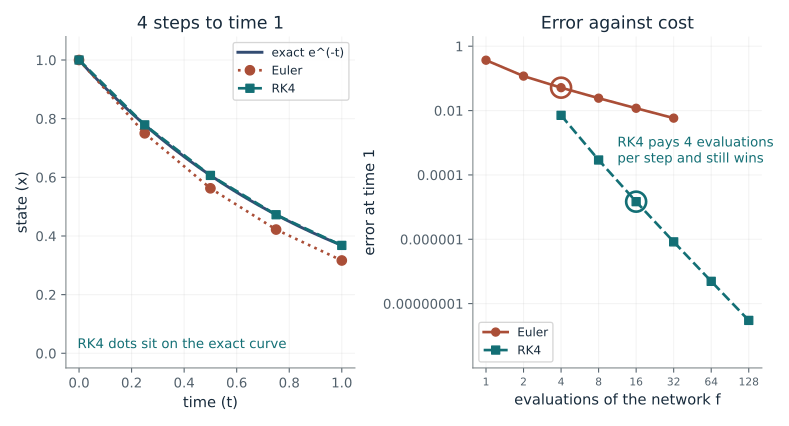
Number of steps: 4 · Horizontal axis of the error plot: evaluations

With 4 steps, Euler is off by 0.0515 and RK4 by 0.0000148. Halving the step roughly halves the Euler error but divides the RK4 error by about 16, so the gap widens quickly.

Euler error at time 1: 0.0515
RK4 error at time 1: 0.0000148
Network evaluations (Euler, RK4): 4, 16
Error ratio (Euler / RK4): 3,490

Why it matters for language models

In a Neural ODE the solver decides how many times the network is evaluated in a forward pass, so the order of the method trades accuracy against compute, much as choosing a layer depth does.

Show the calculation

Step h = 1/4 = 0.25. Euler multiplies by 1 - h = 0.75 per step; RK4 by 1 - h + h^2/2 - h^3/6 + h^4/24 = 0.779. Exact e^(-1) = 0.368. After 4 steps the errors are 0.0515 and 0.0000148.

The equations and symbols

$x_{n+1}=x_n+hf(x_n,t_n)$

$x_{n+1}=x_n+\frac h6(k_1+2k_2+2k_3+k_4)$

$\text{error}_{\text{Euler}}\propto h,\qquad \text{error}_{\text{RK4}}\propto h^4$

h: step size, 1 divided by the number of steps
f: the network that gives the direction of motion
k1..k4: four slope estimates inside one RK4 step
error: distance from e^(-1) at time 1

Where the conclusion applies

Linear test problem with exact answer e^(-1) = 0.368. Each Euler step costs one evaluation of f and each RK4 step four. Orders are asymptotic: they describe how the error shrinks as h becomes small.

Check your understanding: RK4 with 4 steps has error 0.0000148. About what error do you expect with 8 steps?

About 1/16 of it, near 0.00000092. The measured value is 0.00000083, close to this.

Book source: Chapter 12, 12.1.3 Numerical ODE Solvers as Architecture Choices. Illustration C12-D06. Illustration. Book Euler and RK4 formulas and orders. The test problem dx/dt = -x, x(0) = 1 on [0, 1] is a companion choice; errors are recomputed by running both solvers. v39 EPUB / v43 print.

07 / 08

Adjoint gradient against finite differences

From Chapter 12, 12.13.2 Adjoint Gradient Computation: Step-by-Step

How do we get the gradient of a loss through an ODE solve, and how does it compare with nudging the parameter?

The adjoint a(t) carries the loss's sensitivity backward in time. The adjoint is solved backward in time, from t = 1 down to t = 0. Read forward in time, a(t) shrinks exactly as x(t) grows, so their product is constant and the integral equals the closed-form gradient. A finite difference instead compares two loss values, which loses accuracy to curvature when the step is large and to round-off when it is tiny.

Predict first: Does shrinking the finite-difference step always make the gradient more accurate?

Step exponent k (step = 1 / 10^k): 4

112

Target value (y)

Left: state, adjoint and their flat product with area shaded. Right: correct digits against finite-difference step, peaking near 8; adjoint near 11. — **The gradient is the area under the flat product a(t) x(t); one backward solve gets it to about 11 digits, while a finite difference peaks near 8 digits and loses accuracy for smaller steps.**
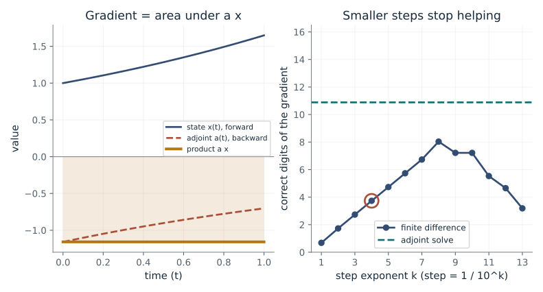
Step exponent k (step = 1 / 10^k): 4 · Target value (y): 2

The adjoint method gets the gradient from one backward solve and agrees with the exact value to 10.9 digits. A finite difference with step 1/10^4 gets 3.7 digits: big steps lose accuracy to curvature, and tiny steps lose it to round-off.

Exact gradient: -1.16
Adjoint solve gradient: -1.16
Finite-difference gradient: -1.16
Correct digits (finite difference, adjoint): 3.7, 10.9

Why it matters for language models

Backpropagating through every solver step stores the whole trajectory; the adjoint method needs one extra backward solve instead, and unlike a finite difference its cost does not grow with the number of parameters.

Show the calculation

x(1) = e^0.5 = 1.649. Gradient = 2 (x(1) - y) x(1) = 2 (1.649 - 2) x 1.649 = -1.16. The adjoint starts at a(1) = 2 (x(1) - y) = -0.703 and a x stays constant at -1.16, so its integral over [0, 1] is the same number.

The equations and symbols

$\dot x=\theta x,\quad \mathcal L=(x(1)-y)^2,\quad \dot a=-\theta a,\quad a(1)=2(x_0e^{\theta}-y)$

$\frac{\partial\mathcal L}{\partial\theta}=\int_0^1a(t)x(t)\,dt=2(x_0e^{\theta}-y)\,x_0e^{\theta}$

$\frac{\mathcal L(\theta+\epsilon)-\mathcal L(\theta)}{\epsilon}$

x(t): state of the scalar Neural ODE, with x0 = 1
theta: the one parameter, set to 0.5
y: target value for x(1)
a(t): adjoint: how the loss changes with the state at time t
epsilon: nudge used by the finite difference, 1 / 10^k

Where the conclusion applies

The forward value x(1) = x0 e^theta is used exactly. The adjoint result comes from a backward 100-step RK4 solve of the state, the adjoint and the running integral. The finite difference is a one-sided difference in 64-bit arithmetic, which carries about 16 digits. Correct digits means minus log10 of the relative error, capped at 16.

Check your understanding: A model has 1,000 parameters. How many solves does a finite-difference gradient need compared with the adjoint method?

About 1,001 forward solves, one baseline plus one nudged run per parameter. The adjoint method needs one forward and one backward solve, whatever the number of parameters.

Book source: Chapter 12, 12.13.2 Adjoint Gradient Computation: Step-by-Step. Illustration C12-D07. Identity. Book worked example (scalar Neural ODE, adjoint integral and closed form). The values x0 = 1, theta = 0.5 and the targets y are companion choices; the finite difference and adjoint solve are computed. v39 EPUB / v43 print.

08 / 08

Stiffness: explicit against implicit Euler

From Chapter 12, 12.5.1 Stiff ODEs and Implicit Solvers

Why does a problem with one very fast direction force tiny steps, even after that direction has died away?

The fast mode vanishes almost immediately in the exact answer, but the explicit method still multiplies it by 1 - h lambda each step. If that factor is below -1, the leftover grows and swamps the slow part. Implicit Euler divides by 1 + h lambda instead, which always shrinks the mode.

Predict first: With rates 1 and 100, how small must the step be for explicit Euler to stay stable, and does implicit Euler have such a limit?

Fast rate (stiffness ratio): 100

10500

Step size (h)

Left: exact curve with implicit Euler on it and explicit Euler leaving the plot. Right: factor per step for each method against h times rate. — **Explicit Euler is stable only for steps below 2 divided by the fastest rate, even when that fast part is long gone; implicit Euler is stable at any step.**
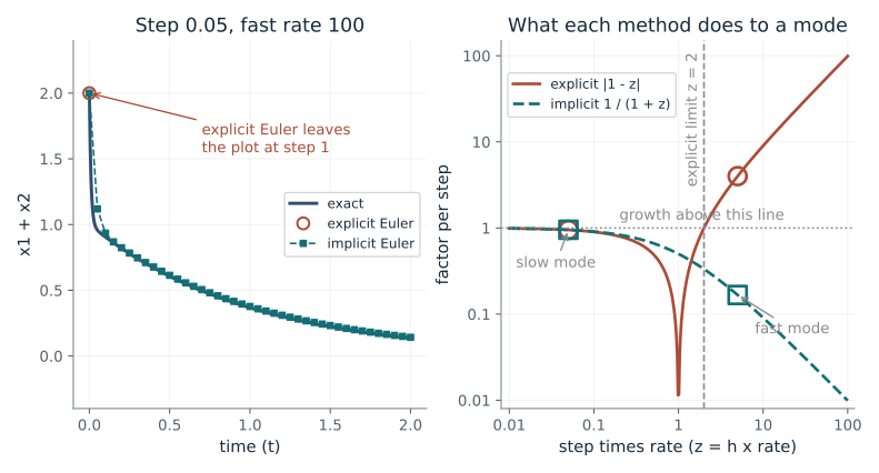
Fast rate (stiffness ratio): 100 · Step size (h): 0.05

With fast rate 100 and step 0.05, explicit Euler blows up because the step 0.05 is above 0.02. Implicit Euler multiplies the fast mode by 0.167 and stays stable at any step. The fast mode dies almost at once in the exact answer, yet it still sets the step size explicit Euler may take.

Stiffness ratio (fast rate / slow rate): 100
Largest stable explicit step (2 / fast rate): 0.02
Explicit factor on the fast mode: -4
Implicit factor on the fast mode: 0.167

Why it matters for language models

A Neural ODE with one very fast direction forces tiny explicit steps, which means many network evaluations; an implicit solver avoids that limit at the cost of solving an equation in every step.

Show the calculation

Fast mode z = h x rate = 0.05 x 100 = 5. Explicit factor 1 - z = -4; stable only if |1 - z| < 1, that is h < 2 / 100 = 0.02. Implicit solves x_new = x_old - h x rate x_new, so x_new = x_old / (1 + z) = x_old x 0.167.

The equations and symbols

$\dot x_j=-\lambda_jx_j,\quad S=\max_j|\lambda_j|/\min_j|\lambda_j|$

$x_{n+1}=(1-h\lambda)x_n\ \text{(explicit)},\qquad x_{n+1}=\frac{x_n}{1+h\lambda}\ \text{(implicit)}$

lambda: decay rate of one mode; here 1 (slow) and the chosen fast rate
S: stiffness ratio: fastest rate divided by slowest rate
h: step size
z: step times rate, h x lambda

Where the conclusion applies

Two independent modes with rates 1 and the fast rate, horizon 2. Explicit Euler is stable only when |1 - h lambda| < 1, that is h < 2/lambda for every mode. The implicit update divides by 1 + h lambda, which is below 1 for every positive step. Linear decay only; nonlinear stiff problems need a solve at each step.

Check your understanding: The fast rate is 500. What is the largest stable explicit step, and how many steps does it need for horizon 2?

The largest step is 2/500 = 0.004, so 2/0.004 = 500 steps. Implicit Euler with h = 0.1 needs only 20 steps and stays stable.

Book source: Chapter 12, 12.5.1 Stiff ODEs and Implicit Solvers. Illustration C12-D08. Illustration. Book formulas for explicit and implicit (backward) Euler and the stiffness ratio. The two-mode test system, both modes starting at 1, is a companion choice. v39 EPUB / v43 print.

Steps approximate continuous decay

Updating can fail to settle

An equilibrium can be sensitive

Numerics can distort conserved energy

One-dimensional flows cannot cross

Euler against RK4: order of a solver

Adjoint gradient against finite differences

Stiffness: explicit against implicit Euler

Bring the idea to a question of your own