Chapter 13 · Scientific ML and Operator Learning

Request the quantity and units, governing relation, domain, material parameters, initial and boundary conditions, observation locations and reference evidence. Return a model-assumption sheet, separate PDE/boundary/initial residuals and a comparison with an analytic case when one applies. For function inputs specify the basis, coefficients and time, and distinguish observation-grid density from model validity. For law discovery require trajectory and derivative provenance, candidate library, column scaling and the precise sparse objective; return fitted coefficients, derivative residuals and an independent trajectory comparison.

Try asking the chapter skill

“This quantitative curve looks plausible. How can I check it mathematically?”

Use mathllms-ch13-scientific-models with the companion's AI skill package. The illustrations below also work on their own.

01 / 08

Watch a sine temperature disperse

From Chapter 13, 13.1.2 Worked Example: 1D Heat Equation

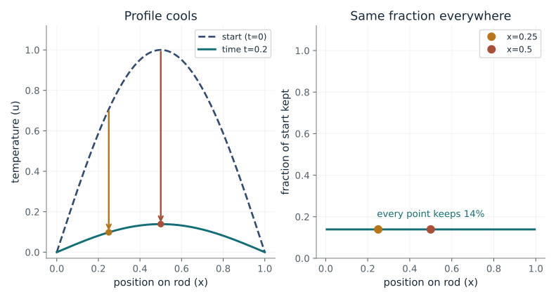
When a rod that starts warm in the middle cools, does every point lose the same share of its heat?

The heat equation says temperature changes at a rate equal to its curvature. For a sine profile the curvature is exactly -pi^2 times the profile itself, so every point decays at the same rate. The ends stay at zero and the start profile is matched at t=0.

Predict first: The middle starts hottest and loses the most degrees. Does it also lose the largest fraction?

Time (t): 0.2

00.5

$Left: sine temperature profile at start and at time t, arrows show drops. Right: flat line of the fraction kept.$

A single sine profile shrinks by one factor, exp(-pi^2 t), at every point, so its shape never changes.
Time (t): 0.2

At t=0.2 the middle has dropped more in absolute terms, but every interior point keeps the same fraction, 0.139, of its starting temperature. A single sine shape only shrinks; it never changes shape.

Fraction kept at every point: 0.139
Temperature drop in the middle: 0.861
Temperature drop at x=0.25: 0.609
Ends of the rod: 0 (held cold)

Why it matters for language models

Splitting a linear map into modes that each shrink by their own factor is the same analysis used for repeated averaging in deep networks, where high-frequency components die first (oversmoothing).

Show the calculation

u(x,t) = exp(-pi^2 t) sin(pi x). exp(-pi^2 x 0.2) = 0.139. Middle: 1 x 0.139 = 0.139. Quarter point: sin(pi/4) = 0.707, so 0.707 x 0.139 = 0.0982. Ratio in both places: 0.139.

The equations and symbols

$\partial_tu=\partial_{xx}u,\quad u(0,t)=u(1,t)=0,\quad u(x,0)=\sin(\pi x)$

$u(x,t)=e^{-\pi^2t}\sin(\pi x)$

x: position on the rod, from 0 to 1
t: time, in normalized units
u: temperature, normalized so the start peak is 1
pi^2: decay rate of the single sine shape

Where the conclusion applies

Exact analytic solution with unit diffusivity, ends held at zero and a sine start profile. Normalized units; no claim about a real material. The ratio is undefined at the two ends (0/0) and is drawn only inside.

Check your understanding: If the start profile were sin(2 pi x) instead, how much faster would it fade?

Four times faster: its curvature is -(2 pi)^2 u = -4 pi^2 u, so it decays like exp(-4 pi^2 t).

Book source: Chapter 13, 13.1.2 Worked Example: 1D Heat Equation. Illustration C13-D01. Illustration. Book equation with companion toy inputs stated in the assumptions; every plotted value is recomputed. v39 EPUB / v43 print.

02 / 08

A smooth candidate can break the rules

From Chapter 13, 13.1.1 Formulation and Architecture

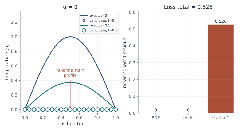
A physics-informed network is scored on three things: the law inside the rod, the end temperatures and the start profile. Can a candidate pass one test and fail another?

The zero function has zero curvature and zero time change, so it satisfies the heat law, and it is zero at the ends. It still fails because it never had the sine start profile. Each candidate fails a different part, which is why the loss keeps the parts apart.

Predict first: A candidate with the wrong decay rate starts exactly at sin(pi x) and is zero at both ends. Which bar catches it?

Candidate function

Start-profile weight (w0)

Left: the zero candidate lies flat while the exact sine starts at 1. Right: three residual bars, only the start bar is nonzero. — **Interior law, end conditions and start profile are separate requirements; a zero in one residual says nothing about the others.**
Candidate function: zero · Start-profile weight (w0): 1

The u = 0 candidate fails the start profile. Each requirement is a separate bar: a candidate can make one residual exactly zero while failing another, so the parts must be reported separately.

Interior law (PDE) residual: 0
End-condition residual: 0
Start-profile residual: 0.526
Weighted loss total: 0.526

Why it matters for language models

Language-model training losses are often sums too, for example a next-token loss plus an auxiliary load-balancing loss in mixture-of-experts layers; a small total can hide one failing term, so each term is logged separately.

Show the calculation

At x=0.5, t=0 the target is sin(pi/2) = 1 and the candidate gives 0, so the squared start error there is (0 - 1)^2 = 1. Averaged over 19 points the start residual is 0.526. Total = 0 + 0 + 1 x 0.526 = 0.526.

The equations and symbols

$\mathcal L=\mathrm{MSE}_{\mathrm{PDE}}+\mathrm{MSE}_{\mathrm{BC}}+w_0\mathrm{MSE}_{\mathrm{IC}}$

$r_{\mathrm{PDE}}=u_t-u_{xx},\qquad r_{\mathrm{IC}}=u(x,0)-\sin(\pi x)$

MSE: mean squared residual on a fixed set of check points
PDE: the heat law u_t = u_xx inside the rod
BC: boundary condition: both ends at 0
IC: initial condition: start profile sin(pi x)
w0: weight on the start-profile term

Where the conclusion applies

Four analytic candidates, no training. PDE checks use 19 interior points j/20 at 20 times from 0.02 to 0.5; end checks use both ends at the same 20 times, pooled into one mean; start checks use the 19 interior points at t=0. Normalization note: the book's worked heat example (13.1.2) averages the sum of both endpoint squares over time, which is twice this pooled mean (0.08 rather than 0.04 for the offset candidate). Compare losses only under the same normalization.

Check your understanding: If the candidate is the exact solution plus 0.2, which requirements fail?

A constant shift changes neither u_t nor u_xx, so the PDE passes. Both ends and the start profile are off by 0.2, giving mean squared residual 0.2^2 = 0.04 each.

Book source: Chapter 13, 13.1.1 Formulation and Architecture. Illustration C13-D02. Illustration. Book equation with companion toy inputs stated in the assumptions; every plotted value is recomputed. v39 EPUB / v43 print.

03 / 08

A function can be the input

From Chapter 13, 13.4.1 PDEs and Solution Operators

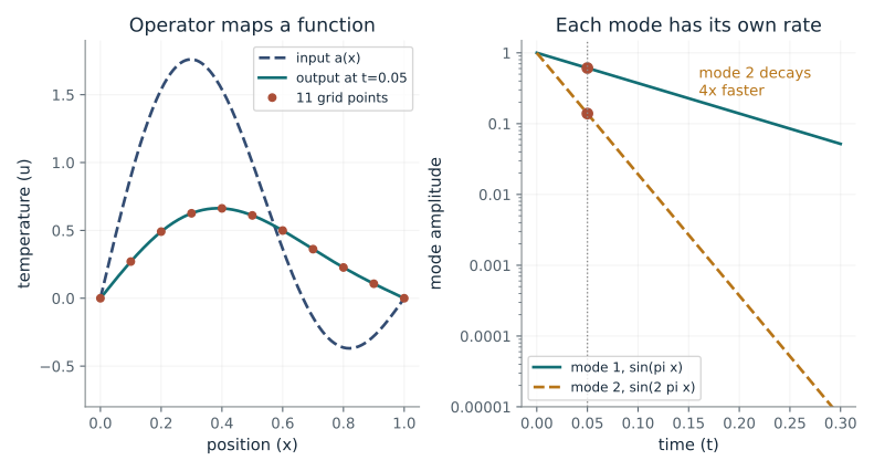
An operator takes a whole curve in and gives a whole curve out. Does sampling the output on a finer grid change the answer?

The input is a whole profile made of two sine modes. The operator multiplies each mode by its own decay factor, so the faster wiggle fades four times faster. The output is a function; a grid only chooses where to look at it.

Predict first: If the display grid goes from 11 to 41 points, does the output value at x=0.25 change?

Time (t): 0.05

00.3

Display grid points

Left: input curve and output curve at t=0.05 with 11 sample dots. Right: two mode amplitudes falling, mode 2 much faster. — **The operator acts on whole functions; each sine mode decays at its own rate k^2 pi^2, and the display grid changes nothing.**
Time (t): 0.05 · Display grid points: 11

The operator takes the whole input curve and returns the whole output curve. At t=0.05 mode 2 has shrunk to 0.139 while mode 1 keeps 0.61. The 11 dots only sample the same curve; changing the grid changes no value.

Mode 1 amplitude: 0.61
Mode 2 amplitude: 0.139
Output at x=0.25: 0.571
Grid points shown: 11

Why it matters for language models

A transformer can be run on longer sequences the way this operator can be sampled on a finer grid; being able to evaluate at a new length is not evidence of being accurate there (the length-generalization question).

Show the calculation

b1 = exp(-pi^2 x 0.05) = 0.61; b2 = exp(-4 pi^2 x 0.05) = 0.139. At x=0.25: 0.61 x sin(pi/4) + 0.139 x sin(pi/2) = 0.61 x 0.707 + 0.139 = 0.571.

The equations and symbols

$\mathcal G_t:a\mapsto u(\cdot,t),\qquad a(x)=\sin(\pi x)+\sin(2\pi x)$

$\mathcal G_t(a)(y)=\sum_{k=1}^{2}b_k(a;t)\,t_k(y),\quad b_k=a_ke^{-k^2\pi^2t},\quad t_k(y)=\sin(k\pi y)$

a: input function: the start temperature profile
G_t: solution operator: maps the start profile to the profile at time t
b_k: amplitude of mode k at time t
t_k(y): basis shape sin(k pi y) at query point y
grid: number of points where the output is displayed

Where the conclusion applies

Exact heat operator restricted to two sine modes with a1 = a2 = 1, unit diffusivity and zero ends. No learned branch or trunk networks; the grid only changes which samples are drawn.

Check your understanding: At what time has mode 2 fallen to 1% of its start while mode 1 still keeps more than 30%?

Mode 2 is at 1% when 4 pi^2 t = ln 100 = 4.61, so t = 0.117. Then mode 1 keeps exp(-pi^2 x 0.117) = 0.32.

Book source: Chapter 13, 13.4.1 PDEs and Solution Operators. Illustration C13-D03. Illustration. Book equation with companion toy inputs stated in the assumptions; every plotted value is recomputed. v39 EPUB / v43 print.

04 / 08

Which law explains a trajectory?

From Chapter 13, 13.6.1 SINDy: Sparse Identification of Nonlinear Dynamics

Sparse regression picks a few terms from a list to explain how a system moves. Can the sparsity penalty erase the true law?

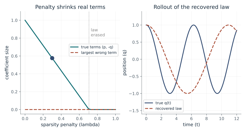
The fit chooses coefficients for each candidate term while paying a price for every nonzero one. With no noise the wrong terms are already zero, so the penalty only shrinks the true terms, which slows the recovered oscillator. Past a threshold it deletes them.

Predict first: Is there a penalty large enough to remove the true terms entirely?

Sparsity penalty (lambda): 0.3

00.8

Measurement noise

Left: true-term size falls as the penalty grows, to zero at 0.707. Right: true cosine versus a slower recovered oscillation. — **An L1 penalty removes wrong terms but also shrinks the right ones; only a rollout shows whether the recovered law still works.**
Sparsity penalty (lambda): 0.3 · Measurement noise: 0

Penalty lambda=0.3, noise 0. The penalty keeps the right terms but shrinks them to 0.576, so the recovered oscillator runs slow and drifts out of phase. A sparse equation that fits is not yet proof of the law: check the rollout.

Size of the true terms: 0.576
Largest wrong term: 0
Nonzero coefficients: 2
Trajectory error on [0,12]: 1.54

Why it matters for language models

Sparse autoencoders used to find features inside language models train with the same L1 penalty, and the same shrinkage makes real features read weaker than they are.

Show the calculation

With unit-scaled, orthogonal library columns and no noise, each true coefficient becomes max(1 - sqrt(2) x lambda, 0) = max(1 - 1.414 x 0.3, 0) = 0.576. Computed here: 0.576. The term vanishes once lambda > 1/sqrt(2) = 0.707.

The equations and symbols

$\dot X\approx\Theta(X)\Xi$

$\min_\beta\frac{1}{2M}\|Y-B\beta\|_F^2+\lambda\|\beta\|_1,\qquad B_j=\Theta_j/\mathrm{RMS}(\Theta_j)$

q, p: position and momentum, q = cos t and p = -sin t
Theta: candidate terms 1, q, p, qp, q^2 - p^2
Y: measured rates dq/dt and dp/dt
beta: coefficients on unit-scaled terms
lambda: sparsity penalty strength
M: number of time samples, 200

Where the conclusion applies

200 uniform samples on [0, 2 pi), analytic rates plus optional Gaussian noise (seed 1304). Coordinate descent solves the normalized L1 objective at every penalty; coefficients are unscaled and the law is integrated from (1, 0) on [0, 12]. Normalization note: the book uses an unnormalized squared residual and penalizes physical coefficients, so its illustrative lambda = 0.1 does not transfer numerically to this scaled objective.

Check your understanding: A colleague reports a recovered law with exactly the right terms. What else should you ask for?

The size of the coefficients and a rollout against held-out data: right terms with shrunken coefficients still predict the wrong motion.

Book source: Chapter 13, 13.6.1 SINDy: Sparse Identification of Nonlinear Dynamics. Illustration C13-D04. Illustration. Book equation with companion toy inputs stated in the assumptions; every plotted value is recomputed. Noise uses seed 1304. v39 EPUB / v43 print.

05 / 08

Keep only the low Fourier modes

From Chapter 13, 13.3.1 Motivation: Discretization-Invariant Convolution

A Fourier neural operator applies its kernel to only the first k_max frequencies. How much does dropping the rest cost?

In Fourier space a convolution is just multiplication, one frequency at a time. Keeping |k| <= k_max discards the rest, and the discarded energy is the error. When the kernel shrinks high frequencies, that energy is tiny.

Predict first: With no smoothing kernel, will keeping 25 modes make the jump in the square wave exact?

Highest mode kept (k_max): 3

125

Kernel

Left: smoothed square wave and its 3-mode truncation. Right: error versus modes kept, smoothing falls fast, identity slowly. — **Truncation error is set by how much the kernel and input carry beyond k_max: a smoothing kernel makes a few modes enough.**
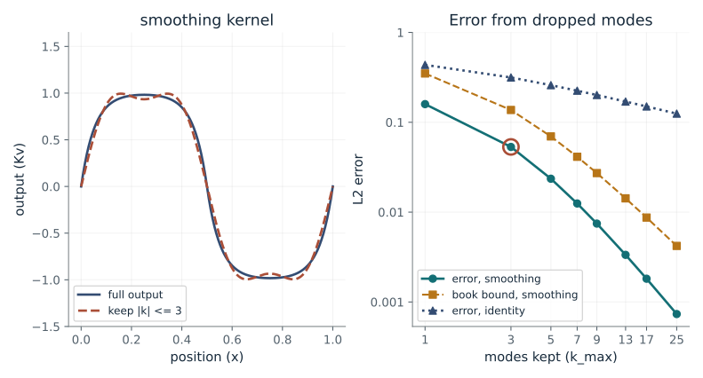
Highest mode kept (k_max): 3 · Kernel: smoothing

Keeping |k| <= 3 leaves an L2 error of 0.0532, under the bound 0.137. The smoothing kernel damps high modes, so the error falls fast as k_max grows.

Nonzero input modes kept: 2
L2 error of truncated output: 0.0532
Book tail bound: 0.137
First dropped mode: 5

Why it matters for language models

Long-convolution sequence layers (state-space and Hyena-style models) also apply kernels through the FFT, and how fast the kernel spectrum decays decides how many frequencies matter.

Show the calculation

The equations and symbols

$\widehat{(\mathcal{K} v)}(k) = \hat{\kappa}(k)\,\hat{v}(k)$

$\|\mathcal{K}v - \mathcal{K}^{(k_{\max})}v\|_{L^2} \leq \sum_{|k| > k_{\max}} |\hat{\kappa}(k)|\,|\hat{v}(k)|$

v: input function, here a square wave on [0, 1]
K: convolution operator with kernel kappa
hat: Fourier coefficient at frequency k
k_max: highest frequency kept
L2: root mean square size of the difference

Where the conclusion applies

Periodic domain [0, 1]; input v(x) = sign(sin 2 pi x), whose odd modes have |v_hat(k)| = 2/(pi k). Fixed kernels stand in for a learned FNO multiplier R[k]: smoothing kappa_hat(k) = 1/(1+(k/3)^2), or identity. Sums run to k = 800,000 (tail below rounding); the full output curve uses modes up to 2001.

Check your understanding: Suppose the kernel were kappa_hat(k) = 1/(1+k^2) instead. Would k_max = 3 be more or less accurate than with the kernel here?

More accurate: at k = 5 the new kernel gives 1/26 = 0.038 versus 0.265 here, so every dropped mode carries less energy.

Book source: Chapter 13, 13.3.1 Motivation: Discretization-Invariant Convolution. Illustration C13-D05. Illustration. Book equation with companion toy inputs stated in the assumptions; every plotted value is recomputed. v39 EPUB / v43 print.

06 / 08

Low notes are learned first

From Chapter 13, 13.1.3 Error Analysis

When a physics-informed network trains, why does it get the broad shape right long before the fine ripples?

In the linearized picture each frequency in the target is learned independently, at its own speed lambda_k. The speed drops roughly with the square of the frequency, so at any moment the network looks like a blurred copy of the target.

Predict first: Once the slow wave is fully learned, roughly how much longer until the k=12 ripple is mostly there?

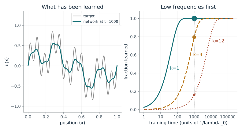
Training time (t): 1000

0100000

Left: network output at t=1000 matches the slow wave but misses ripples. Right: learning curves for k=1, 4, 12. — **Learning speed falls like 1/(1+(2 pi k)^2), so high-frequency detail arrives hundreds of times later than the broad shape.**
Training time (t): 1000

At t=1000 the network has learned 100% of the slow wave, 79% of k=4 and 16% of the fast k=12 ripple. Each frequency learns at rate lambda_0/(1+(2 pi k)^2), so fine detail arrives last.

Learned at k=1: 100%
Learned at k=4: 79%
Learned at k=12: 16%
Slowdown of k=12 versus k=1: 140

Why it matters for language models

Coordinate networks feed positions through sine and cosine features for this reason (Tancik et al.): the book's Fourier-feature fix speeds up the high frequencies that otherwise learn slowest.

Show the calculation

lambda_4 = 1/(1+(8 pi)^2) = 1/633 = 0.00158. Fraction learned = 1 - exp(-lambda_k t) = 1 - exp(-0.00158 x 1000) = 0.794. For k=12: 1 - exp(-0.000176 x 1000) = 0.161.

The equations and symbols

$\lambda_k \approx \lambda_0 \left(1 + (2\pi k)^2\right)^{-1}$

$\text{fraction learned}_k(t) = 1 - e^{-\lambda_k t}$

k: frequency: number of oscillations across [0, 1]
lambda_k: learning speed for frequency k
lambda_0: learning speed of the flat component, set to 1
t: training time, in units of 1/lambda_0

Where the conclusion applies

Linearized training where each frequency's error decays as exp(-lambda_k t) independently; lambda_0 = 1. Target is (sin 2 pi x + sin 8 pi x + sin 24 pi x)/3. The book's formula is approximate; real networks deviate from it.

Check your understanding: Using the book's formula, how much slower is frequency k=10 than the flat component?

About 3,950 times: 1 + (20 pi)^2 = 1 + 3948 = 3949.

Book source: Chapter 13, 13.1.3 Error Analysis. Illustration C13-D06. Illustration. Book equation with companion toy inputs stated in the assumptions; every plotted value is recomputed. The fraction-learned curve is the gradient-flow solution in the linearized (neural tangent kernel) regime. v39 EPUB / v43 print.

07 / 08

Darcy flow in one dimension

From Chapter 13, 13.11.1 Darcy Flow: FNO vs. DeepONet Comparison

For flow through a uniform porous rod, how does the pressure respond to the permeability?

The equation balances the source f against the flux a0 u'. Integrating twice and fixing both ends gives the book's Green formula. For f = 1 it is a parabola whose height is inversely proportional to a0.

Predict first: If permeability triples from 0.5 to 1.5, what happens to the peak pressure?

Permeability (a0): 0.5

0.52.5

Forcing

Left: parabola for a0=0.5 above the a0=1 reference, grid points on it. Right: peak pressure versus a0 falling as 1/a0. — **With constant permeability the solution operator just divides by a0, and the closed form matches an independent grid solve.**
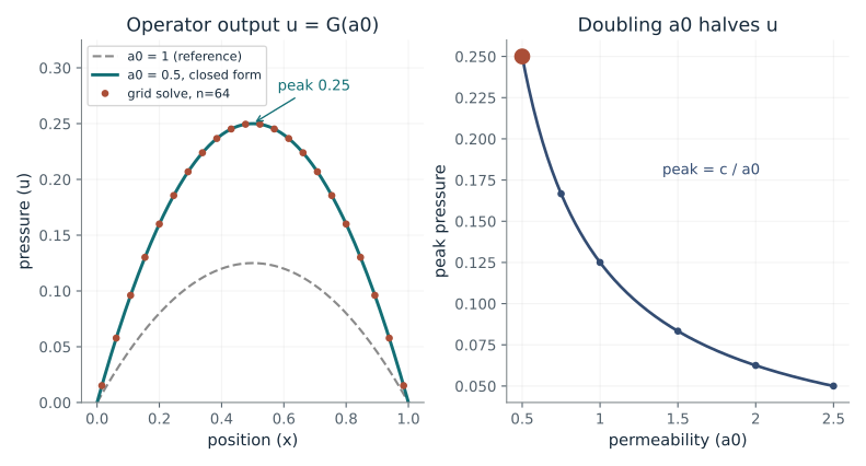
Permeability (a0): 0.5 · Forcing: uniform

With f = 1 and permeability a0=0.5, the pressure peaks at 0.25, which is 2 times the a0=1 curve. A uniform medium only rescales the output by 1/a0; an independent grid solve lands on the closed form.

Peak pressure: 0.25
Peak location (x): 0.5
Largest gap, grid solve vs formula: 0
Peak relative to a0 = 1: 2

Why it matters for language models

Exactly solvable cases like this serve as unit tests for learned surrogates, the way small synthetic tasks with known answers are used to test whether a language model has learned a rule.

Show the calculation

u(x) = x(1-x)/(2 a0). At x=0.5: 0.5 x 0.5/(2 x 0.5) = 0.25/1 = 0.25. Check: u'' = -1/a0, so -(a0 u')' = 1 = f, and u(0) = u(1) = 0.

The equations and symbols

$-(a\,u')' = f\ \text{on}\ [0,1],\qquad u(0)=u(1)=0$

$u(x)=x\int_0^1\frac{1-s}{a_0}f(s)\,ds-\int_0^x\frac{x-s}{a_0}f(s)\,ds$

$f\equiv 1:\quad u(x)=\frac{x(1-x)}{2a_0}$

u: pressure along the rod
a0: constant permeability: how easily fluid passes
f: source term (forcing) pushing fluid in
s: integration variable for source positions

Where the conclusion applies

Constant permeability a0 in the book's range [0.5, 2.5], zero pressure at both ends. The grid solve is a standard second-order finite-difference system on 64 interior points (the book's n = 64), independent of the formula.

Check your understanding: If the source doubles to f = 2 with a0 = 1, what is the peak pressure?

0.25: the operator is linear in f, so the peak doubles from 1/8 to 1/4.

Book source: Chapter 13, 13.11.1 Darcy Flow: FNO vs. DeepONet Comparison. Illustration C13-D07. Identity. Book worked example (closed form for f = 1); the ramp forcing f = x is a companion extension of the same Green formula. Values are recomputed. v39 EPUB / v43 print.

08 / 08

Build an output from p basis shapes

From Chapter 13, 13.2.1 The Branch-Trunk Architecture

A DeepONet writes every output as a weighted sum of p shapes. How many shapes are enough?

The trunk supplies p shapes and the branch says how much of each to use for this input. If the shapes come from the snapshots' singular vectors, the leftover error is set by the singular values that were cut off.

Predict first: Narrow bumps (width 0.06) need how many shapes to get the new output within 5%?

Basis shapes (p): 6

124

Bump width

Left: narrow target bump and a wavy 6-term reconstruction. Right: error versus p, narrow bumps fall slower than wide. — **With p shapes the output lives in a p-dimensional space; error falls as p grows, slowly for sharp outputs and fast for smooth ones.**
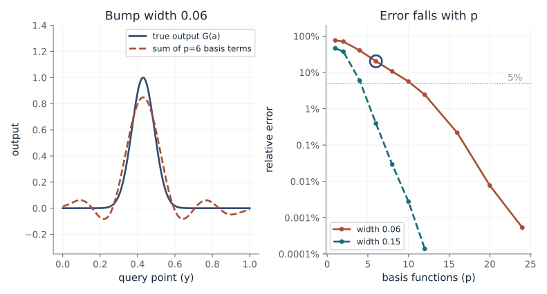
Basis shapes (p): 6 · Bump width: 0.06

With p=6 basis functions the new output is rebuilt with 20.3% error. Narrow bumps need many more basis functions than wide ones: the error is set by how fast the snapshot family's singular values fall.

Basis functions (p): 6
Relative error on a new input: 20.3%
First branch coefficient (b_1): 2.98
Snapshot energy left out: 7.07%

Why it matters for language models

Compressed embeddings make a similar trade: a rank-p basis at best captures what the top p singular values hold and loses the rest. (LoRA also uses low rank, but it learns its update by gradient descent, not by truncating an SVD.)

Show the calculation

Output = b_1 t_1(y) + ... + b_6 t_6(y). Here t_k are the top 6 singular vectors of 41 snapshots and b_k = <t_k, G(a)>; b_1 = 2.98. Relative error = ||G(a) - sum|| / ||G(a)|| = 20.3%.

The equations and symbols

$\mathcal{G}_\theta(a)(y) = \sum_{k=1}^p b_k(a)\, t_k(y) + \beta_0$

$u_i \approx \sum_{k=1}^p \alpha_k^{(i)} \phi_k,\qquad \alpha^{(i)} = \Phi^\top u_i$

a: input function; here it sets where the output bump sits
y: query point where the output is evaluated
t_k: trunk basis shape k (here a POD shape)
b_k: branch coefficient k for this input
p: number of basis shapes
beta_0: offset, zero here

Where the conclusion applies

Outputs are Gaussian bumps exp(-(y-c)^2/(2 w^2)) on 201 points. Trunk shapes are the top p singular vectors (POD) of 41 snapshots with c from 0.1 to 0.9; the branch is the exact projection b_k = <t_k, u>. The test bump at c = 0.43 is not a snapshot. A trained DeepONet learns both parts and need not match POD.

Check your understanding: Why can p = 1 never rebuild bumps centered at different places, however it is chosen?

With one shape every output is a multiple of that shape, so all outputs peak in the same place; moving the peak needs more shapes.

Book source: Chapter 13, 13.2.1 The Branch-Trunk Architecture. Illustration C13-D08. Illustration. Book equation and its POD analogy; the snapshot family is a companion toy and nothing is trained. v39 EPUB / v43 print.

Bring the idea to a question of your own

The chapter skill can adapt the calculations to your inputs. It should identify the assumptions, explain what the result supports, and show what still needs evidence.