Chapter 14 · Bayesian Deep Learning and Uncertainty

01 / 08

Update a belief

From Chapter 14, 14.1.1 Prior, Likelihood, Posterior

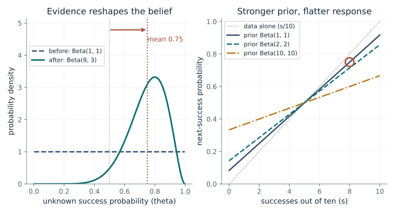
After eight successes and two failures, how likely is the next success, and how much does the starting belief matter?

Bayes weights each possible success probability by how well it explains the data. With a Beta prior the update is just adding counts, so you can see both the whole distribution and its mean change.

Predict first: Will a much stronger prior, Beta(10, 10), pull the answer for eight successes back toward one half?

Prior counts for each side (a = b)

Successes out of ten: 8

010

Left: flat prior and a posterior peaked near 0.8 with its mean marked. Right: next-success probability against successes for three priors. — **The updated mean is a weighted average of the prior mean 0.5 and the observed fraction, and a stronger prior gives the data less weight.**
Prior counts for each side (a = b): 1 · Successes out of ten: 8

8 successes and 2 failures give a next-success probability of 0.75. The prior counts as 2 imagined observations, which pulls the mean 0.05 from the data fraction 0.8 toward 0.5.

Posterior Beta(a, b): Beta(9, 3)
Next-success probability: 0.75
Share of the counts from the prior: 0.167

Why it matters for language models

A pass rate measured on only ten test prompts is this kind of estimate: the prior decides how far a lucky or unlucky streak moves it, the same shrinkage toward a base rate used when comparing models on small evaluation sets.

Show the calculation

a = 1 + 8 = 9, b = 1 + 2 = 3. Mean = a/(a+b) = 9/12 = 0.75. As a weighted average: (2/12) x 0.5 + (10/12) x 0.8 = 0.75.

The equations and symbols

$p(\theta\mid D)\propto p(D\mid\theta)p(\theta)$

$\operatorname{Beta}(a,b)\longrightarrow\operatorname{Beta}(a+s,b+f)$

theta: unknown success probability
a, b: prior counts: imagined successes and failures before any data
s, f: observed successes and failures (ten in total)
mean: next-success probability, a/(a+b) after the update

Where the conclusion applies

Conditionally independent Bernoulli outcomes with a fixed theta, ten observations and a symmetric positive prior. This conjugate example is a specialization, not a network posterior.

Check your understanding: With prior Beta(2, 2) and eight successes out of ten, what is the next-success probability?

Posterior Beta(10, 4); mean 10/14 = 5/7, about 0.714.

Book source: Chapter 14, 14.1.1 Prior, Likelihood, Posterior. Illustration C14-D01. Specialization. Book equation with a disclosed companion toy example. v39 EPUB / v43 print.

02 / 08

Two reasons for uncertainty

From Chapter 14, 14.8.1 Ensemble Diversity and Uncertainty

How much of the total uncertainty is noise inside each model, and how much is the models disagreeing?

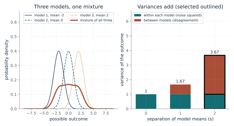
The law of total variance splits the spread of the outcome into two exact pieces. The identity is exact for this equally weighted three-member mixture, and the right panel shows the two pieces stacked.

Predict first: If all three models agree (s = 0), which part of the uncertainty disappears?

Noise inside each model (sd): 1

02.5

Separation of model means (s)

Left: three bell curves centered at -2, 0 and 2 with their wider mixture. Right: stacked variance bars for s = 0, 1, 2. — **Total variance is the noise variance inside the models plus the variance of their means; standard deviations do not add.**
Noise inside each model (sd): 1 · Separation of model means (s): 2

Total variance is 3.67, the sum of 1 (within) and 2.67 (between). Disagreement supplies 0.727 of the total; the rest is noise inside each model.

Within-model variance: 1
Between-model variance: 2.67
Total variance: 3.67
Share from model disagreement: 0.727

Why it matters for language models

Disagreement among several models or sampled answers is a common signal of what a system does not know, and this identity separates it from noise that more models could never remove.

Show the calculation

Within = 1^2 = 1. Between = ((-2)^2 + 0^2 + 2^2)/3 = 2.67. Total = 1 + 2.67 = 3.67, so the standard deviation is 1.91. The divisor is 3 because the three models are equally weighted.

The equations and symbols

$\operatorname{Var}(Y\mid D)=\mathbb E[\operatorname{Var}(Y\mid\theta,D)]+\operatorname{Var}(\mathbb E[Y\mid\theta,D])$

Y: the outcome being predicted
noise: standard deviation of the outcome inside each model
s: separation of the three model means, which are -s, 0 and s
within, between: average noise variance, and variance of the model means

Where the conclusion applies

Equal weights, common conditional variance, finite second moments. The terms are often interpreted as aleatoric and epistemic; these labels do not establish that this mixture captures all real uncertainty.

Check your understanding: If the means are -1, 0, 1 and the within variance is 1, what is the total variance?

Between variance (1 + 0 + 1)/3 = 2/3; total 5/3, not 2.

Book source: Chapter 14, 14.8.1 Ensemble Diversity and Uncertainty. Illustration C14-D02. Specialization. Book equation with a disclosed companion toy example. v39 EPUB / v43 print.

03 / 08

Is eighty percent really eighty percent?

From Chapter 14, 14.5.1 Reliability and Calibration

How does the way forecasts are grouped change the measured calibration gap?

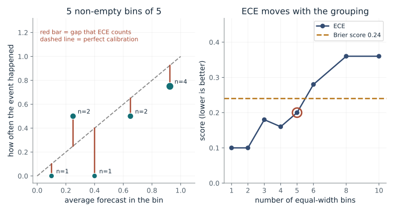
Group forecasts into bins, compare the average forecast with the event rate in each bin, and average the gaps weighted by bin size. Different bins give different gaps from the same ten records, while the Brier score needs no bins.

Predict first: If every one of the ten records is copied three times, will ECE or the Brier score improve?

Equal-width bins: 5

110

Copies of the same records

Left: five bin points against the perfect diagonal with red gap bars. Right: ECE rising with bin count above a flat Brier line. — **ECE depends on how forecasts are grouped and on how many independent records you have; copying records changes the counts but not the score.**
Equal-width bins: 5 · Copies of the same records: 1

Over 10 resolved forecasts, the calibration error (ECE), the bin-weighted average of the gap between each bin's average forecast and its event rate, is 0.2. ECE is 0.2 with 5 bins but ranges from 0.1 to 0.36 across the groupings shown on the right, while the Brier score does not depend on bins.

Records: 10
ECE (weighted gap): 0.2
Brier score: 0.24
Accuracy at a 50 percent cutoff: 0.7

Why it matters for language models

This is how stated probabilities, such as a language model's answer probabilities, are checked against how often the model is right, and why the bins and the number of independent examples must be reported with the score.

Show the calculation

ECE = sum over bins of (count/N) x |event rate - average forecast|. With N = 10, the first non-empty bin has 1 record, so it contributes (1/10) x |0 - 0.1| = 0.01. Adding all 5 bins gives 0.2. Brier = average of (forecast - outcome)^2 = 0.24. Bins are left-closed, right-open, and the last bin includes 1. Empty bins are skipped.

The equations and symbols

$\operatorname{ECE}=\sum_b\frac{|B_b|}{n}|\operatorname{freq}(B_b)-\operatorname{conf}(B_b)|$

B_b: the forecasts that fall in bin b
n: number of resolved records
freq: how often the event actually happened in the bin
conf: average forecast probability in the bin
ECE: expected calibration error, the bin-weighted average of the gap between average forecast and event rate

Where the conclusion applies

Event probabilities in [0, 1], resolved binary outcomes, disjoint equal-width bins with 1 in the last bin. Empty bins have no empirical frequency. Ten fixed illustrative records; duplicated rows are deliberately dependent.

Check your understanding: A bin has 10 forecasts averaging 0.8 and 6 successes. What gap does it contribute if it holds all the records?

|0.6 - 0.8| = 0.2; copying all rows leaves the same gap.

Book source: Chapter 14, 14.5.1 Reliability and Calibration. Illustration C14-D03. Specialization. Book equation with a disclosed companion toy example. v39 EPUB / v43 print.

04 / 08

Turn residuals into an interval

From Chapter 14, 14.7.3 Conformal Regression; finite-sample rank from 14.7.1

Which calibration residual sets the interval half-width, and what if there are too few?

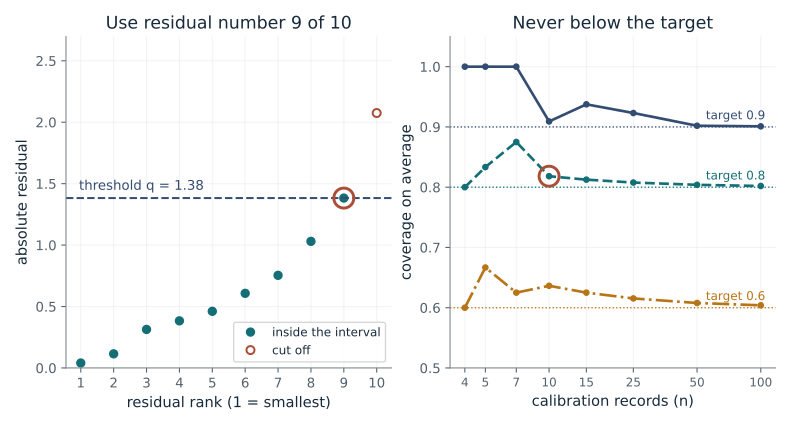
Sort the held-out calibration residuals and pick the corrected rank. The seeded example keeps the prediction fixed at zero so the interval is just [-q, q]. The right panel shows the exact average coverage for every n.

Predict first: What happens when the rank the formula asks for is larger than the number of calibration records?

Calibration records (n): 10

4100

Allowed miss rate (alpha)

Left: ten sorted residuals with the ninth ringed and a threshold line. Right: exact coverage against n for three targets. — **Sort the held-out residuals and take rank ceil((n+1)(1-alpha)); averaged over calibration sets that interval covers at least 1 - alpha, and it is infinite when n is too small.**
Calibration records (n): 10 · Allowed miss rate (alpha): 0.2

Residual number 9 of 10 sets the interval half-width q = 1.38. Averaged over calibration sets the coverage is 0.818, never below the target 0.8. It is above the target because the ceiling rounds the rank up. This one seeded set covered 0.839 of 1,000 fresh cases.

Rank used (k): 9
Threshold (q): 1.38
Coverage on average: 0.818
Covered in 1,000 fresh cases: 0.839

Why it matters for language models

A model that returns a score can be wrapped so its predictions come with intervals or answer sets that hold a stated share of the time, using only held-out examples and no assumptions about the model itself.

Show the calculation

k = ceil((10+1) x (1 - 0.2)) = ceil(8.8) = 9. Take the 9th smallest of the 10 residuals, q = 1.38, so a prediction of 0 gets the interval [-1.38, 1.38]. Coverage = k/(n+1) = 9/11 = 0.818.

The equations and symbols

$k=\lceil(n+1)(1-\alpha)\rceil$

$C(x)=[\hat y(x)-\hat q,\hat y(x)+\hat q]$

n: number of held-out calibration records
alpha: allowed miss rate; the target coverage is 1 - alpha
k: rank of the residual used
q: the kth smallest absolute residual, or infinity if k exceeds n

Where the conclusion applies

Exchangeable calibration and fresh pairs; the prediction and score are fixed independently of the calibration outcomes. Residuals are absolute values of standard normal draws (seed 1404, first n used), so the coverage k/(n+1) is exact for continuous scores. The guarantee is marginal, averaged over calibration sets, not conditional for each individual.

Check your understanding: For n = 4 and alpha = 0.1, is the corrected threshold finite?

ceil(5 x 0.9) = 5 > 4, so q is infinity; an interpolated finite quantile would be wrong.

Book source: Chapter 14, 14.7.3 Conformal Regression; finite-sample rank from 14.7.1. Illustration C14-D04. Specialization. Book equation with a disclosed companion toy example; conformal simulation seeds 1404 and 2404. v39 EPUB / v43 print.

05 / 08

Fit a curve and know where you are unsure

From Chapter 14, 14.13.1 Gaussian Process Regression: A Complete Example (formulas from 14.2.1)

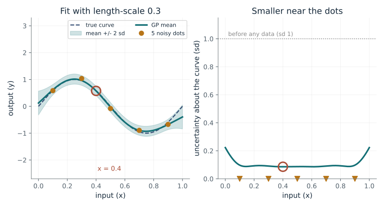
A Gaussian process fits a curve through five noisy dots. Where is it confident, and what sets that?

The kernel says how much one input tells you about another. The posterior mean blends the dots by those weights, and the posterior variance shrinks wherever a dot is close enough to inform it.

Predict first: If the length-scale shrinks to 0.05, so dots 0.2 apart barely relate, what happens to the band between the dots?

Length-scale (ell): 0.3

0.051.2

Assumed noise variance

Left: a smooth curve through five dots with a narrow band, true sine dashed. Right: uncertainty dipping to near 0 at each dot. — **A GP is confident only near its data, and how far that confidence reaches is set by the length-scale, not by the dots' values.**
Length-scale (ell): 0.3 · Assumed noise variance: 0.01

At x = 0.4 the GP predicts 0.575 with sd 0.0861; the true value is 0.588. Neighbouring dots share a kernel value of 0.801, so each dot informs a stretch of the curve and the band narrows near the dots.

GP mean at x = 0.4: 0.575
True value at x = 0.4: 0.588
Uncertainty (sd) at x = 0.4: 0.0861
Largest sd on the curve: 0.223

Why it matters for language models

A model that must say "I do not know" on unfamiliar inputs needs this behaviour, and it shows that stated uncertainty comes from modelling choices such as the length-scale as well as from the data.

Show the calculation

k(0.4, x_i) = exp(-(0.4 - x_i)^2 / (2 x 0.3^2)) for the dots at 0.1, 0.3, 0.5, 0.7, 0.9 gives 0.607, 0.946, 0.946, 0.607, 0.249. Mean = k* (K + 0.01 I)^-1 y = 0.575. Variance = 1 - k* (K + 0.01 I)^-1 k* = 0.00741, so sd = 0.0861.

The equations and symbols

$\mu_*(x_*)=k_*^\top(K+\sigma_n^2I)^{-1}y$

$\sigma_*^2(x_*)=k(x_*,x_*)-k_*^\top(K+\sigma_n^2I)^{-1}k_*$

$k(x,x')=\exp\left(-\frac{(x-x')^2}{2\ell^2}\right)$

ell: length-scale: how far apart two inputs can be and still inform each other
sigma_n^2: noise variance the model assumes in the dots
K: table of kernel values between the five dots
k*: kernel values between the new input and each dot
sd: square root of the posterior variance

Where the conclusion applies

Zero-mean GP with unit amplitude, inputs x = 0.1, 0.3, 0.5, 0.7, 0.9 and one fixed set of responses. The noise variance setting is what the model assumes; the dots themselves do not change. The band shows uncertainty about the curve, not about a new noisy observation. The sd depends only on input locations, kernel and noise variance, never on the responses.

Check your understanding: For length-scale 0.3, what do the GP mean and sd become at x = 3, far outside the dots?

The nearest dot is 2.1 away, so every kernel value is about exp(-24.5), nearly 0. The mean returns to the prior mean 0 and the sd to the prior sd 1.

Book source: Chapter 14, 14.13.1 Gaussian Process Regression: A Complete Example (formulas from 14.2.1). Illustration C14-D05. Illustration. Book worked example: five inputs, RBF kernel, length-scale 0.3 and noise variance 0.01. The book leaves the five responses unspecified, so the responses here are sin(2 pi x) plus one seeded noise draw (seed 1401, sd 0.1), a companion choice. v39 EPUB / v43 print.

06 / 08

Choose the next experiment

From Chapter 14, 14.13.4 Bayesian Optimization on a Synthetic Function (acquisition functions in 14.10.2)

When every evaluation is expensive, how does a Gaussian process decide where to look next?

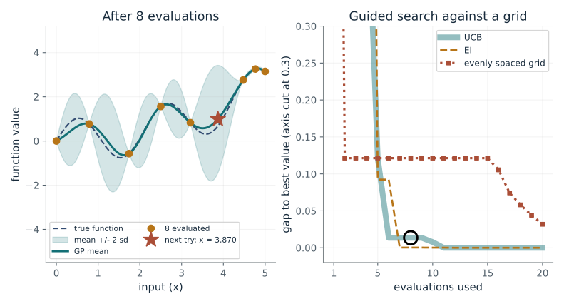
At each step the GP gives a mean and an sd for every candidate. The acquisition function turns those into one score, and the best-scoring point is evaluated next. Large beta favours unexplored places; small beta favours places already known to be good. Exact ties go to the larger x.

Predict first: After 20 evaluations, will the guided search or 20 evenly spaced points sit closer to the true maximum?

Evaluations used: 8

120

Acquisition rule

Scoring each point by its mean plus a bonus for uncertainty sends evaluations to promising or unexplored places, and on this function it reaches the maximum in 11 tries.
Evaluations used: 8 · Acquisition rule: UCB

UCB is 0.0135 below the maximum, closer than an evenly spaced grid of 8 (0.121). The star is the point it would try next.

Best x found so far: 4.765
Gap to the best value: 0.0135
Gap for an evenly spaced grid, same budget: 0.121
Next evaluation at x: 3.870

Why it matters for language models

Choosing which setting to try next when each trial is a costly training run, such as a learning rate or a data mix, uses the same trade-off between exploiting what looks good and exploring what is unknown.

Show the calculation

UCB(x) = mean(x) + sqrt(beta) x sd(x), with beta = 4 so sqrt(beta) = 2. The largest value is at x = 3.870, where 0.991 + 2 x 1.22 = 3.42. Gap = best possible value 3.27 - best found 3.26 = 0.0135.

The equations and symbols

$a^{\text{UCB}}_t(x)=\mu_t(x)+\sqrt{\beta_t}\,\sigma_t(x)$

$a^{\text{EI}}_t(x)=(\mu_t(x)-f^*)\Phi(Z)+\sigma_t(x)\phi(Z),\quad Z=\frac{\mu_t(x)-f^*}{\sigma_t(x)}$

mu: GP mean: current best guess of the function
sigma: GP sd: how unsure that guess is
beta: uncertainty weight in the book's UCB; here beta = 4, so the bonus is 2 sd
f*: best value found so far
UCB, EI: upper confidence bound and expected improvement scores

Where the conclusion applies

Exact (noise-free) evaluations, zero-mean GP with RBF kernel, candidates on 1,001 evenly spaced points, no point evaluated twice. The gap is measured against the best candidate point, and the grid baseline uses n evenly spaced points snapped to the candidates. This is one smooth one-dimensional function, so it does not show that guided search always wins.

Check your understanding: If beta is raised from 4 to 9, does UCB favour exploiting known good points or exploring uncertain ones?

Exploring: sqrt(beta) multiplies the sd, going from 2 to 3, so uncertain places get a bigger bonus.

Book source: Chapter 14, 14.13.4 Bayesian Optimization on a Synthetic Function (acquisition functions in 14.10.2). Illustration C14-D06. Illustration. Book worked example: maximize sin(3x) + 0.1 x^2 on [0, 5]; the book reports a maximum near x = 4.8 after T = 20 evaluations. Kernel length-scale 0.5, amplitude 2, beta = 4 (a bonus of 2 sd) and the start at x = 2.5 are companion choices. v39 EPUB / v43 print.

07 / 08

Fix overconfidence with one number

From Chapter 14, 14.5.3 Temperature Scaling

A classifier is right 68 percent of the time but sounds 85 percent sure. Can one number fix that?

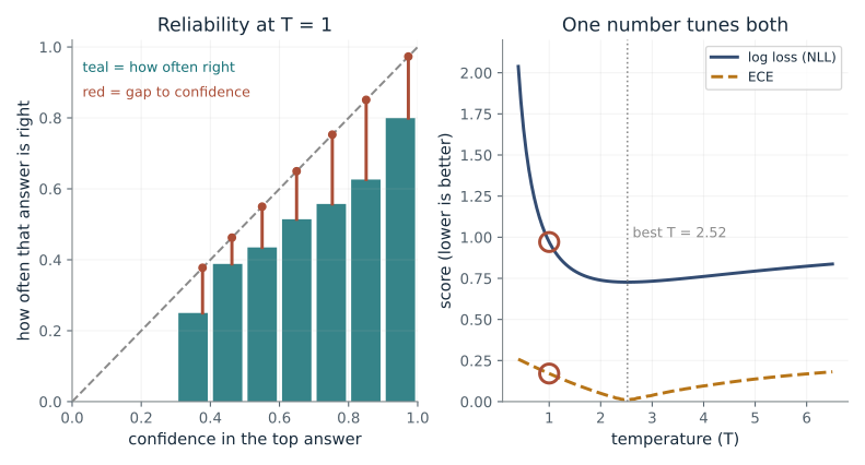
A larger T squeezes the scores together so the softmax spreads probability more evenly. The ranking of the scores is unchanged, so accuracy stays put, while the best T is found by minimizing log loss on held-out cases.

Predict first: Will dividing all scores by T = 2.5 change which class the model picks, and will its confidence match its accuracy?

Temperature (T): 1

0.56

Left: reliability bars far below the diagonal at T = 1. Right: log loss and ECE curves with their minimum near T = 2.5. — **Dividing every score by one temperature T keeps each class ranking, and the T that minimizes log loss brings confidence close to accuracy.**
Temperature (T): 1

At T = 1 the average confidence is 0.849 while the answers are right 0.678 of the time: overconfident by 0.171. Dividing the scores by T never changes which class wins, so accuracy stays 0.678.

Log loss (NLL): 0.971
ECE (10 bins): 0.171
Average confidence: 0.849
Accuracy: 0.678

Why it matters for language models

Dividing logits by T before the softmax is the same operation as the sampling temperature of a language model, here used to make the stated probabilities honest rather than to change the style of the output.

Show the calculation

Take three scores (4, 1, 0). Softmax of scores/T with T = 1: exp(4/T) = 54.6, exp(1/T) = 2.72, exp(0) = 1, so the top answer gets 54.6/(54.6 + 2.72 + 1) = 0.936. Best T minimises the log loss on 3,000 held-out cases: T* = 2.52.

The equations and symbols

$\tilde p(y=c\mid x)=\operatorname{softmax}(z(x)/T)_c$

$\mathbb E[z_y-\textstyle\sum_j\tilde p_jz_j]=0$

z: raw scores (logits) the network gives to each class
T: temperature: one number dividing every score
NLL: negative log-likelihood of the true labels, the log loss
ECE: bin-weighted average of the gap between confidence and accuracy over 10 bins

Where the conclusion applies

Three classes. True scores are normal with sd 1.5, labels are drawn from their softmax, and the network reports 2.5 times those scores, so it is overconfident by construction and the ideal T is near 2.5. Confidence means the top-class probability and ECE uses 10 equal-width bins. The fitted T is the NLL minimizer on these same cases, which is a toy shortcut; real use needs a separate validation set.

Check your understanding: A classifier is right 70 percent of the time but averages 95 percent confidence. Should the fitted T be above or below 1, and does accuracy change?

Above 1, to soften the probabilities. Accuracy stays 70 percent because dividing scores by a positive number never changes their order.

Book source: Chapter 14, 14.5.3 Temperature Scaling. Illustration C14-D07. Illustration. Book equation and first-order condition; the classifier is a companion toy (3,000 held-out cases, seed 1405). v39 EPUB / v43 print.

08 / 08

Why leapfrog, and how big a step

From Chapter 14, 14.4.1 MCMC for Posterior Sampling (HMC and the leapfrog integrator)

Hamiltonian Monte Carlo simulates a rolling particle. How large a step can the integrator take before its energy drifts?

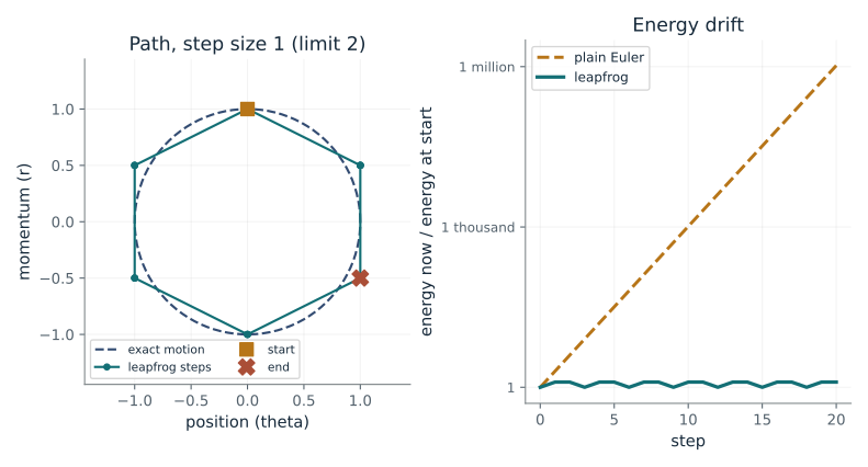
Leapfrog alternates half-kicks to the momentum with a full drift of the position. Unlike plain Euler it keeps the path on a closed loop, so energy wobbles but never drifts, until the step is large enough that the loop itself breaks.

Predict first: Is there a largest safe step size for the leapfrog? Try going just past 2.

Step size (epsilon): 1

0.12.1

Steps taken

Left: leapfrog points on a closed loop near the exact circle. Right: Euler energy exploding while leapfrog energy stays near 1. — **For a bowl-shaped target the leapfrog keeps energy within a fixed factor, 1/(1 - step^2/4), of its start for any step below 2, while plain Euler multiplies energy by 1 + step^2 every step.**
Step size (epsilon): 1 · Steps taken: 20

With step size 1 the leapfrog path stays on a closed loop and its energy never exceeds 1.333 times the start. Plain Euler drifts to 1.05 million times the start after 20 steps.

Highest energy / start (leapfrog): 1.250
Chance of accepting the end point: 0.882
Plain Euler: energy at end / start: 1.05 million
Step size limit for this target: 2

Why it matters for language models

Sampling from a neural-network posterior only works if the step size keeps the simulated energy under control; the same kind of stability limit governs how large a learning rate gradient descent can take.

Show the calculation

Target U = theta^2/2, so the gradient is theta. Start (theta, r) = (0, 1), energy 0.5. Half-kick: r = 1 - (1/2) x 0 = 1. Drift: theta = 0 + 1 x 1 = 1. Half-kick: r = 1 - (1/2) x 1 = 0.5. Energy after one step = (1^2 + 0.5^2)/2 = 0.625. Acceptance probability = min(1, exp(-(energy at end - 0.5))) = 0.882.

The equations and symbols

$r_{t+\epsilon/2}=r_t-\tfrac{\epsilon}{2}\nabla U(\theta_t)$

$\theta_{t+\epsilon}=\theta_t+\epsilon M^{-1}r_{t+\epsilon/2}$

$r_{t+\epsilon}=r_{t+\epsilon/2}-\tfrac{\epsilon}{2}\nabla U(\theta_{t+\epsilon})$

theta: position, standing for the weights
r: momentum of the imaginary particle
U: potential energy; here theta^2/2, a bowl
eps: step size
M: mass, set to 1

Where the conclusion applies

One dimension, unit mass, U = theta^2/2 so the gradient is theta, and the start is theta = 0, r = 1 (energy 0.5). Energy is H = (theta^2 + r^2)/2. The stability limit 2 holds for this unit curvature; other targets have other limits. The acceptance chance uses the Metropolis rule min(1, exp(-change in energy)) at the final point.

Check your understanding: For the same target, do step 0.5 with 40 steps and step 1 with 20 steps cover the same total time, and which has the smaller energy swing?

Both cover time 20. Step 0.5 has the smaller swing: its energy stays within 1/(1 - 0.0625) = 1.07 times the start against 1.33 for step 1.

Book source: Chapter 14, 14.4.1 MCMC for Posterior Sampling (HMC and the leapfrog integrator). Illustration C14-D08. Illustration. Book leapfrog equations; the bowl-shaped target U = theta^2/2 is a companion toy with an exact solution. v39 EPUB / v43 print.

Update a belief

Two reasons for uncertainty

Is eighty percent really eighty percent?

Turn residuals into an interval

Fit a curve and know where you are unsure

Choose the next experiment

Fix overconfidence with one number

Why leapfrog, and how big a step

Bring the idea to a question of your own