Identify the kind of change first. Numerical perturbations, population shifts and interventions need different assumptions and support different conclusions.
“Does this comparison show that changing X would improve Y?”
Use mathllms-ch15-robustness-causality with the companion's AI skill package. The illustrations below also work on their own.
Small input changes, large consequences
From Chapter 15, 15.1.1 Adversarial Examples; 15.1.2 Attack Methods
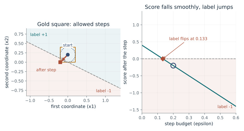
How small a step can change the predicted label?
The score is a smooth function, so a tiny step changes it by a tiny amount. The label is only its sign, so a tiny step is enough to flip it when the score is close to 0.
Predict first: Two inputs get the same step of size 0.2. One has score 0.4 and the other score 1.0. Which keeps its label?
Step budget (epsilon): 0.2 · Starting position (x1): 0
What happens: The input with score 1.0 keeps its label: a step of 0.2 lowers the score only to 0.4. The input at score 0.4 needs only budget 0.133 to flip, so the margin, not the step alone, decides.
A step of size 0.2 moves the score from 0.4 to -0.2, so the label flips from +1 to -1. The score changed by a small, smooth amount; the label jumps as soon as the score crosses 0, which happens at budget 0.133.
- Score at the start
- 0.4
- Score after the step
- -0.2
- Label
- +1 to -1
- Smallest budget that flips the label
- 0.133
Image and text classifiers return a label from a smooth score. Adversarial examples exploit the gap between a small change in score and a jump in label, which is why the margin matters.
Show the calculation
Score = x1 + 2 x2 = 0 + 2 x 0.2 = 0.4. The best step against the score is (-0.2, -0.2), so the score changes by -0.2 - 2 x 0.2 = -0.6, giving -0.2. The label flips once 3 x budget passes the score: budget 0.4 / 3 = 0.133. In the ordinary (2-norm) sense the step has length sqrt(2) x 0.2 = 0.283; the score can move by at most sqrt(5) x 0.283 = 0.632.
The equations and symbols
- f(x)
- score x1 + 2 x2; the label is its sign
- delta
- the step added to the input
- epsilon
- largest allowed change in each coordinate
- L
- sqrt(5), how fast the score can change
Prescribed linear score, true label +1. The step moves each coordinate by epsilon against the score (the sign of the gradient), which is the exact worst case for a linear score in the infinity norm. Nonlinear models need not have this exact worst case.
Check your understanding: A model scores an input 0.5 and each coordinate may move by 0.1 against a score x1 + 2 x2. Does the label flip?
Book source: Chapter 15, 15.1.1 Adversarial Examples; 15.1.2 Attack Methods. Illustration C15-D01. Specialization. Disclosed numerical toy specialization; every plotted value is recomputed. Fixed linear score with weights (1, 2); exact arithmetic, no sampling. v39 EPUB / v43 print.
A certificate has a defined scope
From Chapter 15, 15.4 Certified Robustness; 15.6 threshold example
What can a limited set of noisy votes actually certify?
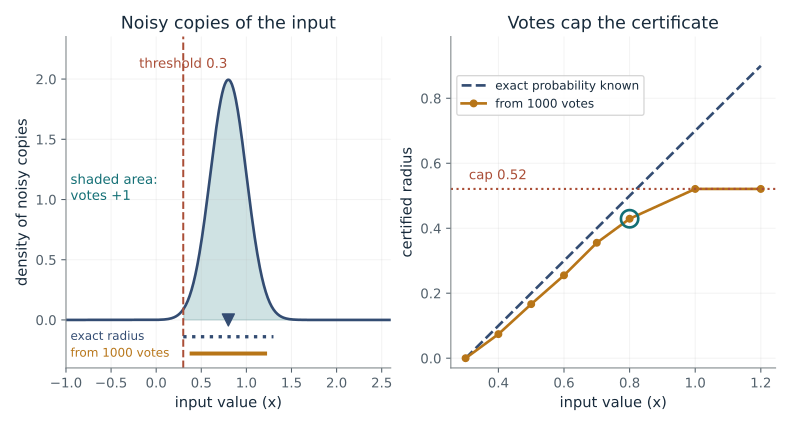
Smoothing certifies the majority vote of noisy copies, not the original classifier. When the probability comes from a finite number of votes, we must use a lower bound, and a finite number of votes can only prove a probability below 1.
Predict first: If almost every noisy copy votes +1, can 1000 votes certify any radius we like?
Original input (x): 0.8 · Noise size (sigma): 0.2
What happens: No. The exact radius is 0.9, but 1000 unanimous votes can only prove a probability near 0.9954, which caps the radius at 0.52.
993 of 1000 noisy copies vote +1. Using the 99% lower bound 0.9841 instead of the raw fraction gives a certified radius of 0.429, a little under the exact 0.5. The certificate covers the smoothed classifier only.
- Chance a noisy copy votes +1
- 0.9938
- Lower bound used (99% sure)
- 0.9841
- Certified radius
- 0.429
- Radius if p were known exactly
- 0.5
Randomized smoothing is a way to certify a classifier against small input changes. How large a certificate you can claim depends on how many noisy samples you draw.
Show the calculation
Exact: p = Phi((0.8 - 0.3) / 0.2) = Phi(2.5) = 0.9938, radius = 0.2 x 2.5 = 0.5. From votes: 993 of 1000 gives a lower bound 0.9841, radius = 0.2 x Phi^-1(0.9841) = 0.2 x 2.146 = 0.429.
The equations and symbols
- sigma
- size of the Gaussian noise added to the input
- p_A lower
- a lower bound on the chance a noisy copy votes +1
- Phi inverse
- turns a probability into a number of standard deviations
- r
- radius around the input where the vote cannot change
Threshold classifier +1 when x > 0.3, Gaussian noise, candidate class +1. A positive radius needs a lower bound above 0.5. The estimate uses a one-sided 99% Clopper-Pearson bound for 1000 seeded votes. The certified interval is open.
Check your understanding: With the same threshold and sigma = 0.2, what is the largest radius that 1000 unanimous votes can certify?
Book source: Chapter 15, 15.4 Certified Robustness; 15.6 threshold example. Illustration C15-D02. Specialization. Disclosed numerical toy specialization; every plotted value is recomputed. The certificate estimation uses seed 1502 and 1000 votes. v39 EPUB / v43 print.
The average changes with the population
From Chapter 15, 15.12.1 Types of Distribution Shift
Can average error rise while each group stays unchanged?
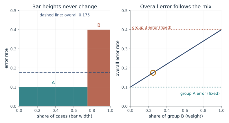
This example changes only the mix of groups and keeps each group's error fixed, so the cause of the average change is visible. The overall error is a weighted average.
Predict first: If group B becomes more common, does either group necessarily get worse?
Share of group B: 0.25
What happens: No. Group B is now 75% of cases and the overall error is 0.325 instead of 0.175, yet group A is still at 0.1 and group B at 0.4.
Group B makes up 25% of cases, so the overall error is 0.175. Each group keeps its own error (0.1 and 0.4); the average moves only because the mix of people changes.
- Share of group B
- 0.25
- Overall error
- 0.175
- Worst group present
- 0.4
- Change from an all-A population
- 0.075
A model evaluated on a new user population can look worse or better only because the mix of cases changed, so a headline number should always be paired with per-group numbers.
Show the calculation
Overall = 0.75 x 0.1 + 0.25 x 0.4 = 0.075 + 0.1 = 0.175.
The equations and symbols
- pi_g
- share of group g in the population; shares add to 1
- R_g
- error rate inside group g, held fixed
- R_test
- overall error rate
Two fixed groups with errors 0.1 and 0.4. Changing those errors would be a different experiment. No estimate of a real population is implied.
Check your understanding: At equal group shares, what are the overall error and the worst-group error?
Book source: Chapter 15, 15.12.1 Types of Distribution Shift. Illustration C15-D03. Specialization. Disclosed numerical toy specialization; every plotted value is recomputed. Exact weighted average of two fixed group error rates; no sampling. v39 EPUB / v43 print.
Observing is different from intervening
From Chapter 15, 15.10.3 Confounders and Adjustment Formulas
Why might observed and adjusted comparisons differ?
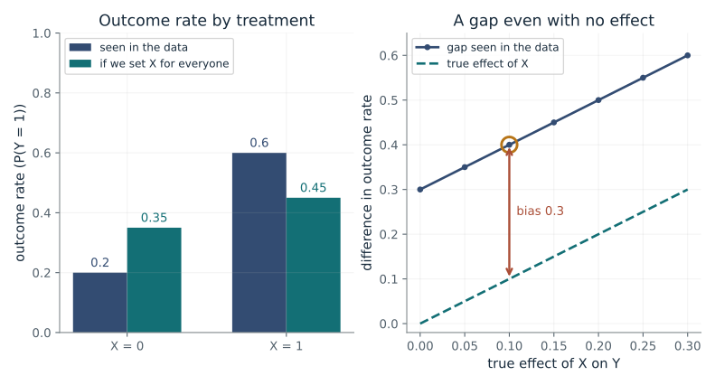
Looking at people who chose X selects a different mix of Z than people who did not. Setting X for everyone uses the same mix of Z for both choices.
Predict first: Can the gap in the data stay large when the true treatment effect is zero?
True effect of X: 0.1 · Share with Z = 1: 0.5
What happens: Yes. With zero true effect the data still show 0.5 against 0.2, a gap of 0.3, because treated cases mostly have Z = 1. Adjustment gives equal rates of 0.35.
People who took X show a gap of 0.4, but setting X for everyone with the same mix of Z gives a gap of only 0.1. The extra 0.3 comes from Z, which raises the outcome and also makes X more likely.
- Gap seen in the data
- 0.4
- Gap if X were set for everyone
- 0.1
- Bias from the common cause Z
- 0.3
- Share with Z = 1
- 0.5
Learned systems pick up whatever predicts the outcome, including a common cause. A model that "finds X helpful" in logs does not show that adding X changes the result.
Show the calculation
Z occurs with probability 0.5; P(X=1 | Z=0) = 0.2 and P(X=1 | Z=1) = 0.8. Outcome rates without X are 0.1 and 0.6, X adds 0.1. Seen: P(Y=1 | X=1) = 0.6, P(Y=1 | X=0) = 0.2. Adjusted: 0.5 x 0.2 + 0.5 x 0.7 = 0.45 against 0.5 x 0.1 + 0.5 x 0.6 = 0.35.
The equations and symbols
- X
- treatment, 1 if taken
- Y
- outcome, 1 if it occurs
- Z
- common cause of X and Y, measured
- do(X=x)
- set X to x for everyone, whatever Z is
Assumed graph Z to X, Z to Y, X to Y, no other confounders, consistency, and positive treatment chance (0.2 or 0.8) in both strata. Observational data alone do not prove these assumptions.
Check your understanding: At Z share 0.5 and effect 0, what are the gap in the data and the adjusted gap?
Book source: Chapter 15, 15.10.3 Confounders and Adjustment Formulas. Illustration C15-D04. Specialization. Disclosed numerical toy specialization; every plotted value is recomputed. Exact enumeration of a stipulated binary joint distribution; no sampling. v39 EPUB / v43 print.
The front door works around a hidden cause
From Chapter 15, 15.10.3 Confounders and Adjustment Formulas
Can we find the effect of X on Y when the common cause is never measured?
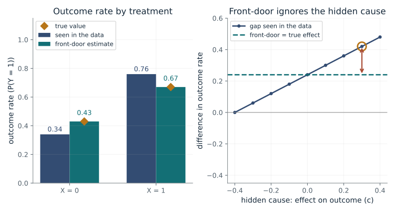
If X reaches Y only through a measured mediator M, and U does not touch M, the effect can be built in two pieces: how X moves M, and how M moves Y after averaging over X. Neither piece needs U.
Predict first: Could the gap in the data point the opposite way from the true effect?
Hidden cause on outcome (c): 0.3 · How much X moves M (s): 0.8
What happens: Yes. The true effect is +0.12 but the gap in the data is -0.12: a hidden cause that lowers the outcome and raises treatment reverses the sign. The front-door estimate still gives +0.12.
The gap in the data is 0.42 but the true effect is 0.24; the difference comes from the hidden cause U. The front-door estimate recovers the true effect from the observed X, M and Y alone.
- Gap seen in the data
- 0.42
- Front-door estimate of the effect
- 0.24
- True effect in the model
- 0.24
- Bias of the seen gap
- 0.18
Auditing a model's effect on outcomes often means a mediator you can measure is the only handle; this shows when such a route is valid and how far a plain comparison can mislead.
Show the calculation
Inner sums: P(Y=1 | m=0) averaged over X = 0.4, over m=1 = 0.7. With P(M=1 | X=1) = 0.9: 0.1 x 0.4 + 0.9 x 0.7 = 0.67. With P(M=1 | X=0) = 0.1 the X = 0 value is 0.43. Effect = 0.3 x (0.9 - 0.1) = 0.24.
The equations and symbols
- U
- hidden common cause of X and Y, never observed
- M
- mediator: X acts on Y only through M
- c
- how strongly U moves the outcome
- do(x)
- set X to x for everyone
Fully stipulated binary model: U is a fair coin; P(X=1 | U) = 0.2 + 0.6 U; P(M=1 | X) = 0.1 + s X; P(Y=1 | M, U) = 0.4 + 0.3 M + c (U - 0.5). U is hidden from the formula. The three front-door conditions hold by construction.
Check your understanding: Suppose M were affected by U as well. Would the front-door formula still be valid?
Book source: Chapter 15, 15.10.3 Confounders and Adjustment Formulas. Illustration C15-D05. Specialization. Disclosed numerical toy specialization; every plotted value is recomputed. Exact enumeration of a stipulated binary joint distribution; no sampling. v39 EPUB / v43 print.
A predictor that holds up where the copy flips
From Chapter 15, 15.9 Worked Example: IRM Identification, A Linear Example
Why does a model that wins in training fail when a spurious feature changes?
Ordinary training uses whatever predicts best on the pooled data, including a spurious copy that agrees with the causal feature in most training cases. The invariant predictor uses only the feature whose relation to the outcome is the same in every environment.
Predict first: As the training mix becomes more lopsided, does the error in environment 2 grow?
Share from environment 1: 0.9 · Blur on the causal feature (tau): 0.5
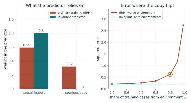
What happens: Yes. At 99% from environment 1, ordinary training puts weight 0.81 on the copy: error 0.024 in environment 1 but 2.7 in environment 2, against 0.21 in both for the invariant predictor.
With 90% of training cases from environment 1, ordinary training leans on the spurious copy (weight 0.32). It scores 0.11 in environment 1 but 0.63 in environment 2, where the copy flips sign. The invariant predictor ignores the copy and scores 0.21 in both.
- ERM weight on the spurious copy
- 0.321
- ERM error, environment 1
- 0.106
- ERM error, environment 2
- 0.628
- Invariant error, either environment
- 0.21
Language models can pick up spurious cues in training text (a topic that co-occurs with a label). Invariance across data sources is a way to ask whether a cue holds beyond one source.
Show the calculation
The causal feature is seen with blur 0.5, so the invariant weight is 1 / (1 + 0.5^2) = 0.8. Its error in either environment is 1.01 - 1/(1 + 0.5^2) = 0.21. ERM solves the 2 by 2 normal equations for the 90% / 10% mix and gets weights (0.594, 0.321).
The equations and symbols
- x_c
- causal feature, seen with blur tau
- x_s
- spurious copy of x_c; sign flips between environments
- tau
- blur: size of the noise on the causal feature
- share
- fraction of training cases from environment 1
Follows the book setup: y = x_c + noise, environment 1 has x_s = x_c + noise, environment 2 has x_s = -x_c + noise, noise variance 0.01. Companion variant: the model sees the causal feature with blur tau, otherwise ordinary training would ignore the copy. Exact population formulas, no sampling. The book's fitted values come from its own run. This shows the target of IRM, not the IRMv1 optimizer. Note on the book: under the book's stated setup, where y depends only on x_c, ordinary training already gives a spurious weight near 0, so both ordinary training and IRM give w_s near 0 there. A spurious effect needs the copy to track y, as in this demo, where the model sees only a blurred x_c.
Check your understanding: With share 0.5, which weights does ordinary training choose?
Book source: Chapter 15, 15.9 Worked Example: IRM Identification, A Linear Example. Illustration C15-D06. Illustration. Follows the book's two-environment example; the causal-feature blur is a companion variant. Exact population formulas, no sampling. The book's fitted values (ordinary training w_s about 0.78, IRM about 0.02) are not reproduced here: they do not follow from its stated setup, where both give w_s near 0. v39 EPUB / v43 print.
Group weights chase the hard groups
From Chapter 15, 15.17 Worked Example: Group DRO, Waterbirds Minimax Dynamics
How do the weights on groups change when one group keeps losing?
Group DRO raises the weight of groups with higher loss by multiplying by an exponential of the loss and renormalizing. Repeating the step with the same losses keeps shifting weight toward the worst group.
Predict first: After one round the two hard groups hold about 52% of the weight. With the same losses, does that stop near half?
Update rounds: 1 · Update step (eta): 0.1
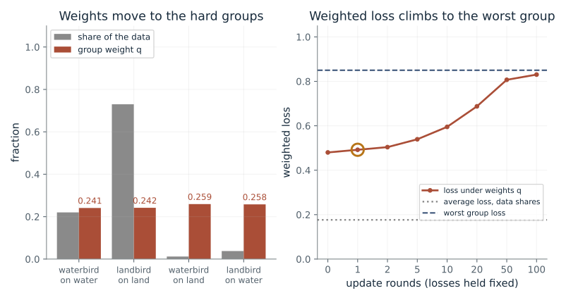
What happens: No. With the losses held fixed the weight keeps flowing to the highest-loss group, waterbirds on land, which holds about 92% after 100 rounds.
After 1 round the two hard groups hold 51.7% of the weight, though they are 5% of the data. The loss under these weights is 0.492, against 0.176 under the data shares, and heads toward the worst group's 0.85. Real training would lower the hard groups' losses, which this fixed-loss view leaves out.
- Weight on the two hard groups
- 51.7%
- Their share of the data
- 5.0%
- Weight on waterbirds on land
- 25.9%
- Loss under the weights
- 0.492
Training on average loss can hide a failing minority group. Reweighting toward worst-performing groups is one way to make a model attend to rare slices of data.
Show the calculation
q_g is proportional to exp(0.1 x 1 x loss_g). Losses (0.12, 0.15, 0.85, 0.80) give exponents (0.012, 0.015, 0.085, 0.08). Exponentials (1.012, 1.015, 1.089, 1.083) sum to 4.199, so q = (0.241, 0.242, 0.259, 0.258).
The equations and symbols
- q_g
- weight on group g, adding to 1
- eta
- step size of the weight update
- L_g
- current loss on group g
- t
- update round
The book's four group losses (0.12, 0.15, 0.85, 0.80), eta 0.1 for one round, uniform start. Rounds beyond the first hold the losses fixed, which is a simplification: real training lowers a group's loss as its weight grows. Data shares 22%, 73%, 1.2%, 3.8% follow the usual Waterbirds split; the book gives only the last two.
Check your understanding: Why do the weights not run away to a single group in real training?
Book source: Chapter 15, 15.17 Worked Example: Group DRO, Waterbirds Minimax Dynamics. Illustration C15-D07. Specialization. Disclosed numerical toy specialization; every plotted value is recomputed. Deterministic weight updates with fixed losses; no sampling. v39 EPUB / v43 print.
Interval bounds are safe but can be loose
From Chapter 15, 15.5.1 Interval Bound Propagation
Can we prove that no small input change flips the label?
Interval bound propagation pushes a box of inputs through the network layer by layer, using the center and a half-width built from absolute weights. The result is guaranteed to contain every possible output, but it ignores how the layers cancel each other.
Predict first: Is the bound also too wide for a network with a single hidden layer?
Allowed change (epsilon): 0.6 · Hidden layers: 2
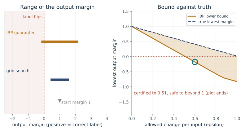
What happens: No. With one hidden layer IBP is exact: both the bound and the true lowest margin are 0.16, so it certifies the label. The gap appears only when layers are stacked.
IBP can only promise a margin of -0.176, below 0, so it cannot certify the label, yet the true lowest margin is 0.412 and the label is safe. The bound is valid but 2 times too wide.
- Starting margin
- 1
- Lowest margin IBP guarantees
- -0.176
- Lowest margin found by grid search
- 0.412
- Verdict
- IBP cannot certify; label is safe
Certified training for language and vision models uses cheap bounds like this one. Looser bounds certify less, so tightness decides how much robustness can be proven.
Show the calculation
Layer 1, unit 1: center = 0.7 x 0.5 + 0.7 x 0.2 + 1 = 1.49; half-width = (0.7 + 0.7) x 0.6 = 0.84. Later layers repeat this with absolute weights, so half-widths keep adding. Output margin interval: [-0.176, 2.18]. True range by grid search: [0.412, 1.59].
The equations and symbols
- l, u
- lower and upper bound on each input of a layer
- mu
- center of the output interval
- r
- half-width of the output interval
- epsilon
- allowed change in each input coordinate
Small fixed ReLU network with 2 hidden units per layer, weights 0.7 and -0.7, bias 1, output the first unit plus an offset making the starting margin 1. The true range is found by an 81 by 81 grid search inside the input box. A failed certificate is not evidence of a flip.
Check your understanding: A single linear layer has weights (0.7, 0.7) and inputs within 0.1 of their centers. What half-width does IBP give?
Book source: Chapter 15, 15.5.1 Interval Bound Propagation. Illustration C15-D08. Specialization. Disclosed numerical toy specialization; every plotted value is recomputed. Deterministic interval arithmetic plus an 81 by 81 grid search; no sampling. v39 EPUB / v43 print.
Bring the idea to a question of your own
Identify the kind of change first. Numerical perturbations, population shifts and interventions need different assumptions and support different conclusions.
The chapter skill can adapt the calculations to your inputs. It should identify the assumptions, explain what the result supports, and show what still needs evidence.