Chapter 16 · Scaling Laws, In-Context Learning, and Abstract Foundations

01 / 08

Read a power law honestly

From Chapter 16, 16.1 Empirical Scaling Laws;16.1.5 The Chinchilla Scaling Law

Why does total loss stop looking like a straight line, and does the slope we care about change?

A power law describes the part of the loss that more resources can remove. On log axes that part is a straight line, but adding a constant floor bends the total away from it. Subtracting the floor brings the straight line back.

Predict first: Raise the floor from 0 to 1. Will the slope of the excess loss change?

Speed of improvement (alpha): 0.5

0.21

Loss floor (E)

Left: total loss against N for floors 0, 0.2 and 1; higher floors bend flat. Right: excess loss is a straight line with a slope marker. — **A floor flattens the visible slope of total loss, but the excess above the floor keeps the same slope.**
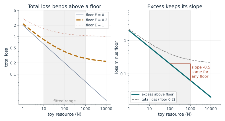
Speed of improvement (alpha): 0.5 · Loss floor (E): 0.2

The excess above the floor falls with slope -0.5 whatever the floor. The total loss, which is what a plot of raw loss shows, reads a flatter slope of -0.25 over the fitted range because the floor never shrinks.

Slope of excess loss: -0.5
Apparent slope of total loss (N from 10 to 1000): -0.25
Total loss at N=100: 0.4
Excess factor when N doubles: 0.707

Why it matters for language models

Scaling-law plots of language-model loss are read for a slope; a floor of unavoidable error (the randomness in text itself) means the raw-loss slope understates how fast the reducible part is falling.

Show the calculation

Excess at N=100 is 2/100^0.5 = 0.2; adding the floor 0.2 gives total 0.4. Doubling N multiplies the excess by 2^(-0.5) = 0.707. A straight-line fit of log total against log N over 10 to 1000 has slope -0.25, not -0.5.

The equations and symbols

$L(N,D)=E+AN^{-\alpha}+BD^{-\beta}$

E: loss floor that more resources cannot remove
A: size constant, set to 2 here
N: toy resource amount (model size or data)
alpha: how fast the excess shrinks

Where the conclusion applies

Assumed illustrative law with A = 2 and the other resource held in the floor; not fitted empirical data. The shaded 10-1000 range is a teaching convention. No inference about a current product or future performance is supported.

Check your understanding: A fitted total-loss curve gives slope -0.1 over its range. Can you say the reducible loss falls at rate 0.1?

Not without the floor. If the floor is large, the reducible part can fall much faster than the total suggests; fit the excess above a stated floor.

Book source: Chapter 16, 16.1 Empirical Scaling Laws;16.1.5 The Chinchilla Scaling Law. Illustration C16-D01. Specialization. Book formulas with explicitly illustrative constants and stipulated toy models, not measured product performance. v39 EPUB / v43 print.

02 / 08

Spend a fixed resource wisely

From Chapter 16, 16.1.5 The Chinchilla Scaling Law

With a fixed compute budget, how should it be split between model size and data?

Making the model larger leaves less budget for data. Each side lowers the loss by a power law, so the total has a single lowest point on the budget line. At that point one more unit of compute helps the model and the data equally.

Predict first: Even with alpha = beta = 0.5 the best split is not equal (A = 2, B = 1). If the data exponent beta drops to 0.2, which way does the best split move?

Data exponent (beta): 0.5

0.21

Model exponent (alpha)

Left: loss along the fixed-compute line with the best size and the equal split marked. Right: the budget line with best splits for each beta. — At fixed compute there is one best split. Where it falls depends on both exponents and on the constants A and B: equal exponents need not give an equal split (alpha = beta = 0.5 gives N = 63, D = 16 here, because A = 2 and B = 1).
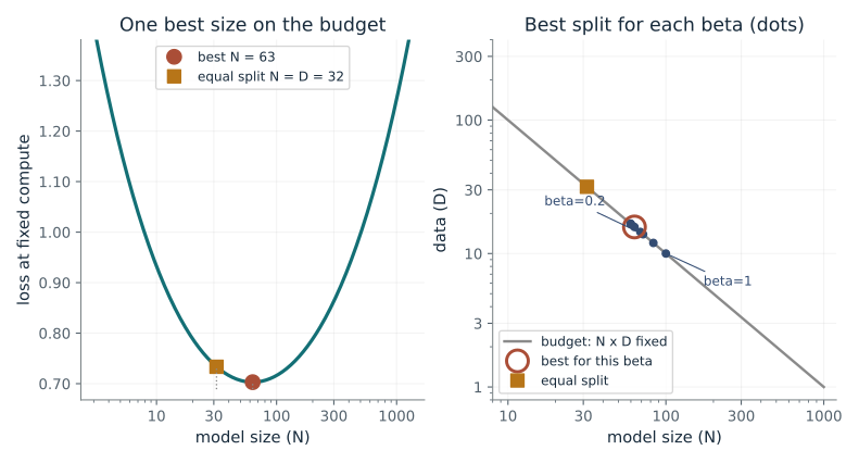
Data exponent (beta): 0.5 · Model exponent (alpha): 0.5

With data exponent 0.5 and model exponent 0.5, the best split of the budget is N = 63.2, D = 15.8, which beats the equal split by 0.0305 in loss. The best split moves along the budget line as beta changes.

Best model size N: 63.2
Best data D: 15.8
Loss at the best split: 0.703
Loss at equal split: 0.733

Why it matters for language models

Choosing how many tokens to train a model of a given size on is exactly this trade; an unbalanced split wastes compute on the resource that is already saturated.

Show the calculation

K = C/6 = 1000. N* = [(alpha A)/(beta B) K^beta]^(1/(alpha+beta)) = [(0.5 x 2)/(0.5 x 1) x 1000^0.5]^(1/1) = 63.2. D* = K/N* = 15.8. At the best split the two gains match: alpha A/N^alpha = 0.126 and beta B/D^beta = 0.126. Illustrative constants A=2, B=1, floor 0.2; real fits differ.

The equations and symbols

$C=6ND$

$N^*=\left(\frac{\alpha A}{\beta B}(C/6)^\beta\right)^{1/(\alpha+\beta)},\quad D^*=\frac{C}{6N^*}$

C: compute budget, fixed at 6000 toy units
N: model size
D: amount of training data
alpha, beta: how fast model and data improve the loss
A, B: size constants, 2 and 1 here

Where the conclusion applies

Positive exponents and constants, continuous unrestricted N and D, and compute relation C = 6ND. Data caps, integer sizes, actual hardware and deployment costs are outside this toy optimum. Floor E = 0.2.

Check your understanding: If compute is doubled (C = 12000) with alpha = beta = 0.5, how do N* and D* change?

Both grow by the square root of 2, about 1.41 times: N* = sqrt(4 x 2000) = 89.4 and D* = 22.4. Equal exponents split the growth evenly.

Book source: Chapter 16, 16.1.5 The Chinchilla Scaling Law. Illustration C16-D02. Specialization. Book formulas with explicitly illustrative constants and stipulated toy models, not measured product performance. v39 EPUB / v43 print.

03 / 08

Examples change a prediction

From Chapter 16, 16.2.2 Bayesian ICL;16.2.3 Linear-attention one-step GD

How do a few examples reweight the rules a model might be following?

The Bayesian model keeps three candidate rules and shifts weight toward those that fit the examples. The gradient model starts at zero and takes one step along the data. They both use the same examples but need not agree.

Predict first: Two exact examples (1,1) and (2,2) follow y = x. Will an almost noise-free Bayesian match the one-step gradient rule?

Number of examples

Assumed noise in examples: 1

0.252

Left: three candidate lines through example points, thickness showing posterior weight. Right: three predictions at x = 1.5 as bars. — **Bayesian reweighting can settle on the right rule from examples, while one gradient step from zero can land far from it.**
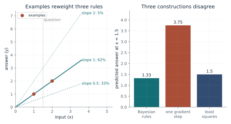
Number of examples: 2 · Assumed noise in examples: 1

With 2 examples and noise 1, the Bayesian answer is 1.33; the one gradient step predicts 3.75 and least squares 1.5. Assumed noise reweights the Bayesian rules; the single step ignores noise.

Weights on slopes 0.5, 1, 2: 33%, 62%, 5%
Bayesian prediction: 1.33
One-step weight: 2.5
One-step prediction: 3.75

Why it matters for language models

Researchers explain in-context learning with two different toy stories, rule selection and implicit gradient descent; the numbers show they make different predictions, so neither can be taken as the whole account.

Show the calculation

One step from zero: w = (1/K) sum y x = 2.5, so the query gives 1.5 x 2.5 = 3.75. Least squares: w = sum xy / sum x^2 = 1, giving 1.5. Bayes: weights are proportional to exp(-sum (m x - y)^2 / (2 x 1^2)) for m = 0.5, 1, 2, then normalized: 0.331, 0.618, 0.051.

The equations and symbols

$p(y^*\mid x^*,D)=\int p(y^*\mid x^*,\theta)p(\theta\mid D)\,d\theta$

$\hat y(x^*)=x^{*T}\left(\frac1K\sum_i y_i x_i\right)$

x, y: an example input and its answer
theta: which rule is true (the slope here)
K: number of examples
x*: the new question, 1.5 here

Where the conclusion applies

Bayesian model: stipulated fixed candidate rules (slopes 0.5, 1, 2) with equal prior and known Gaussian noise. GD model: scalar squared loss normalized by 1/(2K), zero initial weight and one unit step, softmax-free linear attention. Neither is a universal model of deployed ICL.

Check your understanding: Why does the one-step weight (the mean of y x) equal the least-squares slope when there is only the example (1,1)?

With K = 1 and x = 1 the step is y x = 1, and least squares is y x / x^2 = 1. They coincide only when the mean of x^2 equals 1.

Book source: Chapter 16, 16.2.2 Bayesian ICL;16.2.3 Linear-attention one-step GD. Illustration C16-D03. Specialization. Book formulas with explicitly illustrative constants and stipulated toy models, not measured product performance. v39 EPUB / v43 print.

04 / 08

What you reward changes what you get

From Chapter 16, 16.8.2 KL-Constrained Policy;16.12.6 Reward Hacking

Does stronger optimization improve the quality you actually care about?

The best distribution multiplies each starting probability by an exponential of its reward, then renormalizes. A small beta makes that exponential steep. If the reward is not the true goal, the steepest option can be the worst one.

Predict first: Under the proxy reward, will pushing harder (smaller beta) favor the highest-quality option?

Penalty on moving away (beta): 1

0.14

Reward used

Left: reference and tilted probabilities for options A, B, C. Right: expected true quality against beta for the true-quality and proxy rewards. — **Optimizing a proxy harder moves the distribution toward what the proxy likes, which can lower the quality you wanted.**
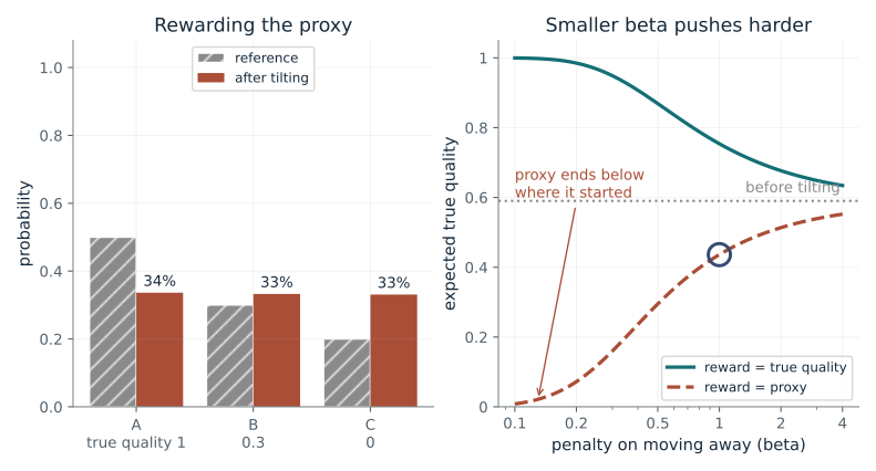
Penalty on moving away (beta): 1 · Reward used: proxy

With penalty beta = 1 the distribution moves 0.0677 nats from the reference and expected true quality becomes 0.436 (was 0.59). The proxy favors C, which has the lowest true quality, so tilting lowers it.

Probabilities of A, B, C: 34%, 33%, 33%
Distance moved from reference (KL, nats): 0.0677
Expected true quality: 0.436
True quality before tilting: 0.59

Why it matters for language models

Reward models for language models are imperfect stand-ins for what people want, so pushing the policy hard against one is how reward hacking appears.

Show the calculation

Each option gets reference x exp(reward/beta). For A: 0.5 x exp(0.1/1) = 0.553; the three values are divided by their sum. Expected true quality = 0.336 x 1 + 0.333 x 0.3 + 0.331 x 0 = 0.436.

The equations and symbols

$p^*(y\mid x)\propto p_{\mathrm{ref}}(y\mid x)e^{r(x,y)/\beta}$

p_ref: starting probabilities: 0.5, 0.3, 0.2
r: the reward being optimized
beta: penalty on moving away from the start; small means push hard
p*: best distribution after tilting

Where the conclusion applies

Finite supported menu, beta > 0, normalized positive reference and fixed toy scores: true quality (1, 0.3, 0), proxy reward (0.1, 0.6, 1). Zero reference probability would remain zero. Toy quality is prescribed, not an estimate of factual correctness.

Check your understanding: If the reward is the same for all options, what is the best distribution?

The starting distribution, for every beta: the common exponential factor cancels in the normalization.

Book source: Chapter 16, 16.8.2 KL-Constrained Policy;16.12.6 Reward Hacking. Illustration C16-D04. Specialization. Book formulas with explicitly illustrative constants and stipulated toy models, not measured product performance. v39 EPUB / v43 print.

05 / 08

Emergence can be a ruler artifact

From Chapter 16, 16.4.2 Are Emergent Capabilities Real?

If every token gets steadily more accurate, why can an exact-match score look like it switches on suddenly?

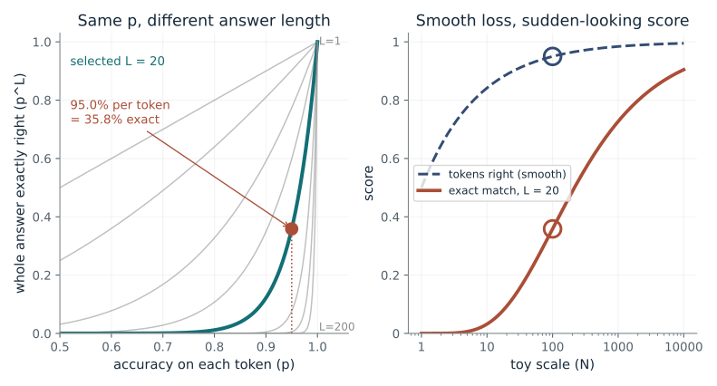
Multiplying L chances that are each slightly below 1 gives a number far below 1. As each chance improves, the product rises slowly at first and then quickly. The shape belongs to the metric, not to the model.

Predict first: At 95% accuracy per token, roughly what share of 50-token answers is exactly right?

Answer length (L tokens): 20

1200

Marked toy scale (N)

Left: exact-match p^L against token accuracy for several lengths. Right: smooth token accuracy and a steeper exact-match curve over scale. — **A score that needs every token right turns smooth token improvement into a steep curve, with no new ability required.**
Answer length (L tokens): 20 · Marked toy scale (N): 100

At N = 100 each token is right 95.0% of the time, yet a 20-token answer is exactly right only 35.8% of the time. Token accuracy improves smoothly; the all-or-nothing score only seems to switch on at large scale.

Accuracy on each token: 95.0%
Whole answer exactly right: 35.8%
Answer length (tokens): 20
Token accuracy needed for 50% exact: 96.59%

Why it matters for language models

Reported jumps in benchmark accuracy for language models can come from the scoring rule; checking token-level or partial-credit scores shows whether the underlying ability changed smoothly.

Show the calculation

Per-token error = 0.5 x N^(-1/2) = 0.5 x 100^(-0.5) = 0.05, so p = 0.95. Exact match needs all 20 tokens right: p^L = 0.95^20 = 0.358. For 50% exact match p must reach 0.5^(1/20) = 0.966.

The equations and symbols

$\text{exact match}=p^{L}$

$p^{L}\ge\tfrac12\iff p\ge 2^{-1/L}$

p: chance that each token is right
L: answer length in tokens
N: toy scale; per-token error is 0.5 / sqrt(N)

Where the conclusion applies

Tokens are right independently with the same probability p, and the score gives credit only when all L are right. Real errors are correlated and vary by token, so p^L is an idealization; the smooth per-token law is assumed, not fitted.

Check your understanding: What per-token accuracy gives a 100-token answer a 50% chance of being exactly right?

0.5^(1/100) = 0.9931, about 99.3%, so very high token accuracy is needed before long exact answers appear.

Book source: Chapter 16, 16.4.2 Are Emergent Capabilities Real?. Illustration C16-D05. Illustration. Book formulas with explicitly illustrative constants and stipulated toy models, not measured product performance. The toy per-token error law 0.5 / sqrt(N) is invented for illustration. v39 EPUB / v43 print.

06 / 08

Five features in two dimensions

From Chapter 16, 16.5.8 Toy Model of Superposition: A Worked Example

When features are rare, can a layer store more of them than it has dimensions?

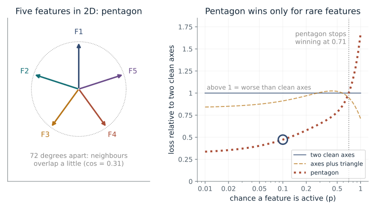
With rare features, an input usually activates one direction, and its small spill onto neighbours costs less than dropping a feature entirely. When many are active together the spills add up and distort every answer.

Predict first: With 80% of features active at once, does packing five directions into two dimensions still beat two clean axes?

Chance a feature is active (p): 0.1

0.020.8

Directions used

Left: five unit arrows in a plane arranged as a pentagon. Right: expected loss against p for three layouts, pentagon lowest for rare features. — **In the pentagon layout, sharing directions beats two clean axes only while features are rare enough that they seldom appear together.**
Chance a feature is active (p): 0.1 · Directions used: pentagon

At p = 0.1 the pentagon layout loses 0.142 against 0.3 for two clean axes, so it wins. Sharing directions costs interference only when several features are active together.

Expected loss, this layout: 0.142
Expected loss, two clean axes: 0.3
Loss added per active feature (small p): 0.191
Pentagon stops winning above p: 0.705

Why it matters for language models

Neurons in language models often respond to several unrelated features; this toy shows why sparse features can be packed into fewer dimensions, which is what sparse autoencoders try to undo.

Show the calculation

Two clean axes: features 3, 4, 5 are never reconstructed, so loss = 3p = 3 x 0.1 = 0.3. This layout, one feature active: total error 0.955 over five features, about 0.955 x p = 0.0955 at small p; exact average over all 32 on/off inputs = 0.142. Pentagon: 10 x cos^2(72 degrees) = 0.955.

The equations and symbols

$\hat x=\mathrm{ReLU}(W^{T}W x)$

$\mathcal L(W)=\mathbb E\Big[\sum_{k=1}^{5}(x_k-\hat x_k)^2\Big]$

W: 2 x 5 matrix; column k is the direction of feature k
x_k: feature k, 1 if active else 0
p: chance each feature is active, independently
ReLU: keeps positive values, zeroes negative ones

Where the conclusion applies

The book fixes five binary features, two dimensions and two clean axes (loss p3 + p4 + p5). The companion adds a tied decoder xhat = ReLU(W^T W x), equal probability p for all features, unit-length directions and an exact average over all 32 inputs. The pentagon (72 degrees apart) is a companion variant; the book draws a triangle for the last three. The book states that no universal threshold follows; the break-even shown holds only for these choices.

Check your understanding: In the pentagon, why is the loss per active feature (at small p) the same for every feature?

By symmetry each direction has two neighbours at 72 degrees with overlap cos 72 = 0.31; the error is 2 x 0.31^2 = 0.19 for each, so five features add up to 0.95 p.

Book source: Chapter 16, 16.5.8 Toy Model of Superposition: A Worked Example. Illustration C16-D06. Illustration. Book formulas with explicitly illustrative constants and stipulated toy models, not measured product performance. v39 EPUB / v43 print.

07 / 08

Why PPO clips the update

From Chapter 16, 16.10.4 PPO: The Clipped Surrogate Objective

What stops a policy from moving too far in one update?

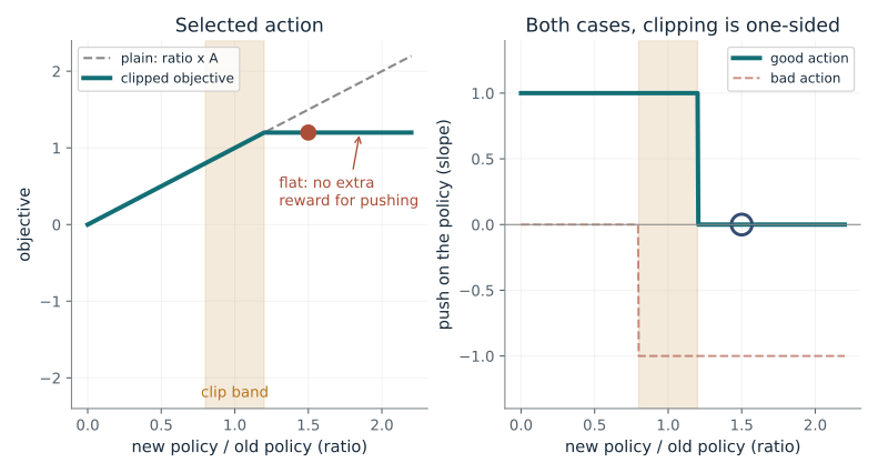
The ratio compares the new policy to the one that collected the data. Taking the smaller of the plain and clipped terms is pessimistic: it ignores improvements that come from large moves, yet it keeps every penalty.

Predict first: A bad action (A < 0) has had its probability raised to 1.5 times the old one. Does clipping stop the push to lower it?

Band half-width (epsilon): 0.2

0.050.4

Action quality

Left: PPO objective against the probability ratio with a shaded clip band. Right: slope of the objective for good and bad actions. — **The clip removes the reward for moving far in the helpful direction, but leaves the penalty for a bad action in place.**
Band half-width (epsilon): 0.2 · Action quality: good action (A = +1)

For a good action the objective stops rising once the ratio passes 1.20, so at 1.5 there is no further push. The update is not allowed to profit from moving far in one step.

Clip band for the ratio: 0.80 to 1.20
Plain objective at ratio 1.5: 1.5
Clipped objective at ratio 1.5: 1.2
Push at ratio 1.5: none (clipped)

Why it matters for language models

This is the rule that keeps reinforcement-learning fine-tuning of language models stable: each batch of samples can only be trusted near the policy that produced it.

Show the calculation

Ratio 1.5, A = +1, eps = 0.2. Plain term: 1.5 x +1 = 1.5. Clipped term: clip(1.5, 0.80, 1.20) x +1 = 1.20 x +1 = 1.2. Objective = min of the two = 1.2.

The equations and symbols

$\rho=\frac{\pi_\theta(a\mid s)}{\pi_{\mathrm{old}}(a\mid s)}$

$L^{\mathrm{CLIP}}=\min\big(\rho\hat A,\ \mathrm{clip}(\rho,1-\epsilon,1+\epsilon)\hat A\big)$

rho: new probability of the action divided by the old
A: advantage: how much better than average the action was
epsilon: half-width of the allowed band around ratio 1
clip: forces the ratio into the band

Where the conclusion applies

One sampled action with a fixed advantage estimate, no KL term and no value-function term. The gradient is taken with respect to the ratio at fixed A; at the corners of the clip band the slope is set to the unclipped value.

Check your understanding: For a good action with eps = 0.1, above what ratio does the update lose all incentive to increase the probability further?

Above 1.1: past that the clipped term is constant at 1.1 x A, so the slope is zero.

Book source: Chapter 16, 16.10.4 PPO: The Clipped Surrogate Objective. Illustration C16-D07. Identity. Book formulas with explicitly illustrative constants and stipulated toy models, not measured product performance. Advantage values of +1 and -1 are illustrative. v39 EPUB / v43 print.

08 / 08

How DPO weighs a preference pair

From Chapter 16, 16.8.3 Direct Preference Optimization

When does one preference pair stop teaching the model anything?

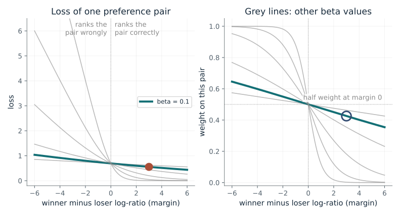
The loss is the negative log of the probability that the model prefers the winner. Its gradient is large when that probability is small and fades as it approaches one, which is the rule that each pair is learned until it is ranked correctly.

Predict first: If the model already ranks a pair correctly (margin 3), does a larger beta make the pair matter more or less?

Sharpness (beta): 0.1

0.052

Margin on this pair (m)

Left: DPO loss against margin for six beta values. Right: gradient weight sigma(-beta m) against margin, with the selected pair circled. — **The weight on a pair is the model's own chance of getting it wrong, and beta sets how quickly that chance falls.**
Sharpness (beta): 0.1 · Margin on this pair (m): 3

With beta = 0.1 the model already ranks the pair correctly (margin 3), the loss is 0.554 and the pair gets weight 0.426. A larger beta saturates sooner: correct pairs stop contributing, wrong pairs keep full weight.

Reward gap (beta x margin): 0.3
Chance model prefers the winner: 57.4%
Loss: 0.554
Weight on this pair: 0.426

Why it matters for language models

DPO trains language models directly on preference pairs; this weight explains why training focuses on pairs the model still ranks wrongly and why beta controls how far the model drifts.

Show the calculation

Reward gap = beta x margin = 0.1 x 3 = 0.3. Loss = -log sigma(0.3) = 0.554. The gradient weight is sigma(-beta m) = sigma(-0.3) = 0.426.

The equations and symbols

$\mathcal L=-\log\sigma(\beta m),\quad m=\log\tfrac{p_\theta(y_w)}{p_{\mathrm{ref}}(y_w)}-\log\tfrac{p_\theta(y_l)}{p_{\mathrm{ref}}(y_l)}$

$\frac{\partial\mathcal L}{\partial m}=-\beta\,\sigma(-\beta m)$

y_w, y_l: the preferred and the rejected response
m: margin: how much more the winner gained than the loser, in log-ratio
beta: sharpness of the preference model
sigma: logistic function, 1 / (1 + e^(-z))

Where the conclusion applies

One preference pair with a given margin m (a free control, not derived from a model). The weight sigma(-beta m) is the exact factor in the gradient, in addition to the constant beta.

Check your understanding: What is the weight on a pair with margin 0, for any beta?

0.5: sigma(0) = 1/2, so an undecided pair always gets half weight, whatever beta is.

Book source: Chapter 16, 16.8.3 Direct Preference Optimization. Illustration C16-D08. Identity. Book formulas with explicitly illustrative constants and stipulated toy models, not measured product performance. v39 EPUB / v43 print.

Read a power law honestly

Spend a fixed resource wisely

Examples change a prediction

What you reward changes what you get

Emergence can be a ruler artifact

Five features in two dimensions

Why PPO clips the update

How DPO weighs a preference pair

Bring the idea to a question of your own