Chapter 17 · The Mathematics of Truth, Error, and Abstention

01 / 08

Estimate the mass of what has not appeared

From Chapter 17, 17.3.1 Missing Mass and the Monofact Rate; 17.3.2 Why the Estimator Works

Can types seen exactly once tell us something about types that the sample has missed?

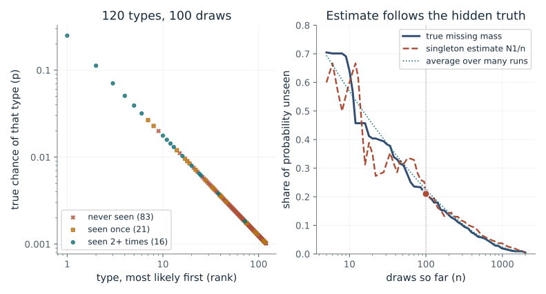
Missing mass adds the true probabilities of types never seen, which ordinary data cannot directly reveal. Good-Turing uses the observable singleton count as a proxy for that hidden mass. The expectation identity explains the estimator's positive bias, while the seeded paths show why one observed estimate can still fall on either side of truth.

Predict first: Increase n with the seed fixed. Must the true unseen mass fall at every step? Must the singleton estimate fall at every step?

Draws so far (n): 100

102000

Reproducible sample (seed)

Left: 120 types by rank, coloured unseen, seen once, seen often. Right: true missing mass and singleton estimate both falling as draws grow. — **The share of once-seen types tracks the hidden mass of unseen types, though a single run can land on either side of it.**
Draws so far (n): 100 · Reproducible sample (seed): 23

With 100 draws, 21 types appear once, so the estimate is 0.21 while the true unseen mass is 0.215. The truth is visible only because this demo lists the whole population; in one run the estimate can land on either side.

Types seen exactly once (N1): 21
Singleton estimate (N1/n): 0.21
True missing mass (known only here): 0.215
Estimate minus truth in this run: -0.005

Why it matters for language models

A language model trained on a long-tailed corpus meets many facts exactly once. The singleton share is the standard way to ask how much of what a model will be asked about it has never effectively seen.

Show the calculation

N1 = 21 types seen once, n = 100, so N1/n = 21/100 = 0.21. 83 types were never seen; adding their true probabilities gives 0.215. On average over many runs the estimate exceeds the missing mass by sum p^2 (1-p)^(n-1), which here equals 0.00125.

The equations and symbols

$M_0=\sum_{x:N_x=0}p(x),\qquad \widehat M_0=\frac{N_1}{n}$

$\mathbb E[M_0]=\sum_x p(x)(1-p(x))^n,\qquad \mathbb E[\widehat M_0]-\mathbb E[M_0]=\sum_x p(x)^2(1-p(x))^{n-1}$

p(x): true chance of type x on one draw
n: number of independent draws so far
N1: number of types seen exactly once
M0: true probability held by types never seen (missing mass)
N1/n: the singleton (Good-Turing) estimate of M0

Where the conclusion applies

Independent draws with replacement from a fixed normalized distribution. The known population lets this demo compute the normally hidden true mass. The finite population can eventually be fully observed, so it does not reproduce an inexhaustible open world. A positive expected bias does not force the realized error to be positive, and missing mass alone is not a hallucination-rate prediction.

Check your understanding: For probabilities (0.5, 0.3, 0.2) and observed counts (2, 1, 0), what are actual missing mass and the singleton estimate?

Only the third type is unseen, so actual missing mass is 0.2. One type occurs exactly once among three draws, giving the estimate 1/3. The quantities need not coincide in a realized sample.

Book source: Chapter 17, 17.3.1 Missing Mass and the Monofact Rate; 17.3.2 Why the Estimator Works. Illustration C17-D01. Estimator and simulation. Book missing-mass and bias identities. Simulation population is explicitly finite: 120 types with p(rank) proportional to rank^-1.15. Seed is a control (7, 23, or 71); curves use prefixes of the same seeded sample. v39 EPUB / v43 print.

02 / 08

Trade answer coverage against error and cost

From Chapter 17, 17.9.1 Coverage and Selective Risk; 17.9.2 The Risk-Coverage Curve; 17.12.1 Scoring Rules That Reward Guessing

When does answering fewer questions improve reliability, and when is abstention worth its cost?

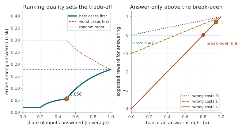
Selective risk divides retained error mass by retained input mass, so adding a band changes both numerator and denominator. Good ranking removes difficult cases first; poor ranking keeps them first and makes the answered subset worse. The reward rule adds a separate choice: how much a wrong answer costs relative to an abstention.

Predict first: At 50% coverage, will answering only part of the inputs still lower the error rate if the ranking is reversed (worst cases first)?

Share of inputs answered (coverage): 0.5

01

How the inputs are ranked

Left: risk against coverage for three rankings, selected point circled. Right: expected reward lines for three wrong-answer costs, break-even at 0.8. — **Answering fewer inputs lowers the error rate only if the ranking sends the hard inputs to the abstain side.**
Share of inputs answered (coverage): 0.5 · How the inputs are ranked: informative

At coverage 0.5 with informative ordering the answered group has error rate 0.056. Its average reward per answer is 0.72 when a wrong answer costs 4, against 0 for abstaining. A group average does not certify any single answer.

Coverage: 50%
Selective risk: 0.056
Errors per 100 original inputs: 2.8
Average reward per answer (wrong costs 4): 0.72

Why it matters for language models

An assistant that declines low-confidence questions is only as reliable as its confidence ranking. This plot is the check: the risk-coverage curve of a real system should look like the teal line, not the terracotta one.

Show the calculation

Risk = (0.2 x 0.02 + 0.3 x 0.08) / 0.5 = 0.056. Chance right = 1 - 0.056 = 0.944. Reward = 0.944 x 1 - 0.056 x 4 = 0.72. Break-even = (0 + 4)/(1 + 4) = 0.8. Within each band the error rate is taken as uniform.

The equations and symbols

$C(\tau)=\Pr(s(X)\geq\tau),\qquad R(\tau)=\Pr(\widehat Y\ne Y\mid s(X)\geq\tau)$

$p\cdot1+(1-p)(-\lambda)\geq u_a\quad\Longleftrightarrow\quad p\geq\frac{u_a+\lambda}{1+\lambda}$

s(X): score that ranks inputs from most to least answerable
C: coverage: share of all inputs we choose to answer
R: risk: error rate among the answered inputs only
p: chance an answer is correct
lambda: cost of a wrong answer (a right answer earns 1)
u_a: reward for abstaining, here 0

Where the conclusion applies

Band errors are uniform within each band for interpolation. Informative ranking keeps low-error bands first; reversed ranking keeps high-error bands first; uninformative ranking samples all bands proportionally. Zero coverage has no conditional risk. Rewards and error rates refer to the stated evaluation population, and group accuracy does not give a verified probability for every individual answer. The control sets coverage directly rather than a score threshold.

Check your understanding: Reproduce the book's risk at retained coverage 0.5. With wrong-answer penalty 4 and abstention reward 0, what probability justifies answering?

Risk is (0.2 times 0.02 + 0.3 times 0.08)/0.5 = 0.056. The break-even is (0 + 4)/(1 + 4) = 0.8. At exactly 0.8, answering and abstaining tie in expected reward.

Book source: Chapter 17, 17.9.1 Coverage and Selective Risk; 17.9.2 The Risk-Coverage Curve; 17.12.1 Scoring Rules That Reward Guessing. Illustration C17-D02. Conditional probability and decision rule. Book population bands: masses (0.2, 0.3, 0.5), with errors (0.02, 0.08, 0.30). Informative ordering is the source example; reversed and uninformative ordering are illustrative comparisons. Reward lines use the book's penalties 0, 1, and 4, with abstention reward 0. v39 EPUB / v43 print.

03 / 08

Follow an answer back to usable evidence

From Chapter 17, 17.10.1 Retrieval-Augmented Marginalization; 17.10.3 The Three-Part Failure Decomposition; 17.10.4 Tools and Proof-Carrying Answers

What does a retrieval probability mean, and which checks still stand between retrieval and a grounded answer?

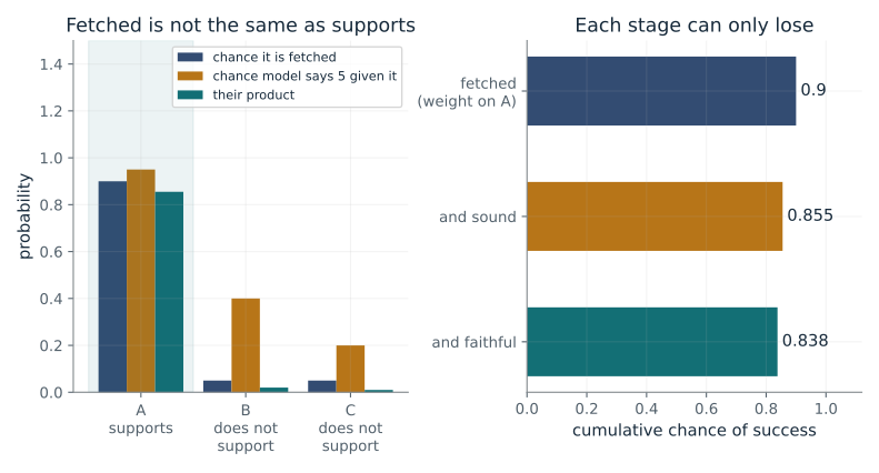
The mixture is a weighted sum of document-conditioned answer distributions. Inspecting the actual source adds a different check: whether it is relevant and whether its content supports the claim. The success chain keeps retrieval, sound evidence, and faithful use separate, so a strong result at one stage is not mistaken for complete reliability.

Predict first: Make retrieval favor the entropy source (C) while the question asks for a vector norm. Can its retrieval weight rise even though its content does not answer the question?

Where retrieval puts its weight

Faithful use, given earlier success: 0.98

0.51

Left: three source documents with retrieval weight, answer chance and product bars; only A supports. Right: cumulative success chain of three stages. — **A source can be fetched often without supporting the claim, and success needs fetch, sound evidence and faithful use in turn.**
Where retrieval puts its weight: favor-evidence · Faithful use, given earlier success: 0.98

The model gives answer 5 a chance of 0.885, but that is a weighted average of invented numbers, not a check. Only source A supports the norm and it is fetched with weight 0.9, so the grounded path succeeds 83.8% of the time.

Chance model answers 5 (mixture): 0.885
Weight on the supporting source A: 0.9
Fully grounded success: 0.838
Chance the grounded path fails: 0.162

Why it matters for language models

Retrieval-augmented assistants cite whatever the retriever returns. This is why a citation or a high retrieval score is not a check: someone still has to open the source and see whether it supports the claim.

Show the calculation

Mixture = 0.9 x 0.95 + 0.05 x 0.40 + 0.05 x 0.20 = 0.885. The real check is sqrt(3^2 + 4^2) = 5 using source A. Grounded success = 0.9 (chance A is fetched) x 0.95 x 0.98 = 0.838; each factor is conditional on the earlier ones, so no independence is assumed.

The equations and symbols

$p(y\mid x)=\sum_z p_\eta(z\mid x)\,p_\theta(y\mid x,z)$

$\Pr(R\cap E\cap F)=\Pr(R)\Pr(E\mid R)\Pr(F\mid R\cap E)$

x, y: the question and an answer
z: a candidate source document
p_eta: retrieval weight: chance the document is fetched
p_theta: model's chance of answering y given the document
R, E, F: retrieval succeeds, evidence is sound, answer is faithful to it

Where the conclusion applies

The mixture sums over a normalized finite source distribution. Model answer probability is not a truth label. In this toy the retrieval weight on source A is also used as the stage-one chance of fetching it, so the chain follows the selected weights; real retrievers need a separate recall estimate. Evidence quality is conditioned on successful recall, and faithfulness on both prior successes; independence is unnecessary. Other paths can produce a correct guess without satisfying the fully grounded event.

Check your understanding: Why is the grounded success rate 0.8379 rather than 0.98 in the default chain, and does multiplying the three factors require independence?

The faithful final stage succeeds only after retrieval and evidence quality have succeeded, so the rate is 0.9 times 0.95 times 0.98 = 0.8379. These are conditional factors from the probability chain rule; independence is not required.

Book source: Chapter 17, 17.10.1 Retrieval-Augmented Marginalization; 17.10.3 The Three-Part Failure Decomposition; 17.10.4 Tools and Proof-Carrying Answers. Illustration C17-D03. Identity and illustrative model. Book mixture identity and conditional success example 0.9 x 0.95 x 0.98 = 0.8379 (the book prints about 0.838), reproduced by the favor-evidence setting with weight 0.9 on source A. The three source documents are real Chapter 1 passages from ch002.xhtml at the named anchors. Retrieval weights (which also set stage-one recall) and document-conditioned answer probabilities (0.95, 0.4, 0.2) are explicitly invented teaching values. v39 EPUB / v43 print.

04 / 08

Generate an option, then recognize it

From Chapter 17, 17.11.1 pass@k and Conditional Sampling; 17.11.2 Best-of-N and Verifier Types

How much can repeated answers help when their errors are related and selection is imperfect?

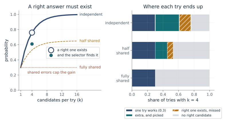
Independent candidates increase the chance that at least one works. An exact checker turns that availability q into a correct accepted answer and abstains when none works. An imperfect selector can miss a correct option, so its overall success is qv. Shared outcomes limit the benefit of repetition; similar answers cannot automatically count as independent confirmation.

Predict first: In the fully shared mode every candidate repeats the same success or failure. Can raising k, even to 16, improve the chance that a right answer exists?

Candidates per try (k): 4

116

How much the candidates share

Left: chance a right candidate exists against k for three sharing levels. Right: stacked bars splitting one try into one-try, extra, missed, none. — **Extra candidates help only as far as their errors are independent, and an imperfect selector wastes part of what remains.**
Candidates per try (k): 4 · How much the candidates share: independent

With 4 candidates a right one exists 76% of the time. The imperfect selector picks a right answer 61% of the time.

A right candidate exists (q): 0.76
Same chance if independent: 0.76
Picked answer is right: 0.61
Gain over a single try: +0.310

Why it matters for language models

Best-of-n sampling and majority voting improve a model only when the sampled answers fail in different ways. Samples from one model often repeat the same mistake, so n agreeing answers are less than n independent confirmations.

Show the calculation

Independent: 1 - 0.7^4 = 0.76. Sharing weight rho = 0: q = 0 x 0.3 + 1 x 0.76 = 0.76. All candidates right: 0.0081. Picked right = 0.0081 + 0.8 x (0.76 - 0.0081) = 0.61. An exact checker would accept q of the batches and be right on every accepted one.

The equations and symbols

$q_{\mathrm{ind}}=1-(1-p)^k,\qquad q_\rho=\rho p+(1-\rho)\left[1-(1-p)^k\right]$

$\Pr(\text{selected correct})=qv,\quad v=\Pr(\text{selector succeeds}\mid\text{a correct candidate exists})$

$C_{\mathrm{exact}}=q,\qquad \Pr(\text{correct}\mid\text{accepted by exact checker})=1\quad(q>0)$

p: chance one candidate is correct, fixed at 0.3
k: number of candidates per try
q: chance at least one candidate is correct
rho: chance a try shares one outcome across all its candidates
v: chance the selector picks a right one when one exists

Where the conclusion applies

The independent formula applies to repeated draws conditional on one fixed prompt. Across heterogeneous prompts, average the per-prompt coverage instead of substituting mean p. The shared model lets a try share one Bernoulli outcome with probability rho; no generic effective-sample shortcut is assumed. An exact checker is taken as sound and complete: it accepts q of the tries and is right on every accepted one; if p = 0 nothing is accepted and its accuracy is undefined. The imperfect selector always answers, succeeds 80% of the time on mixed batches, and succeeds when all candidates are correct.

Check your understanding: At p = 0.3 and k = 2, compare independent availability, exact-checker acceptance and accuracy, and imperfect selected correctness. What changes if p = 0?

Availability is 1 - 0.7 squared = 0.51. The exact checker accepts 51% of batches, returns a correct answer on every accepted batch, and abstains otherwise. Both candidates are correct with probability 0.09; exactly one is correct with probability 0.42. The imperfect selector's success is 0.09 + 0.8 times 0.42 = 0.426, so v is about 0.8353. At p = 0 the exact checker accepts nothing; its conditional accuracy is undefined, not zero or one.

Book source: Chapter 17, 17.11.1 pass@k and Conditional Sampling; 17.11.2 Best-of-N and Verifier Types. Illustration C17-D04. Identity and illustrative dependence model. Book independent-sampling coverage identity and exact qv decomposition. The shared-outcome model, p = 0.3, and 80% selection success on mixed batches are illustrative. All curves and bars are analytic, not simulated. v39 EPUB / v43 print.

05 / 08

How sure is an accuracy number?

From Chapter 17, 17.2.1 Closed-World Statistics

A model answers 90 of 100 questions correctly. What range of true accuracy is reasonable, and why does the textbook formula fail when accuracy is near 100%?

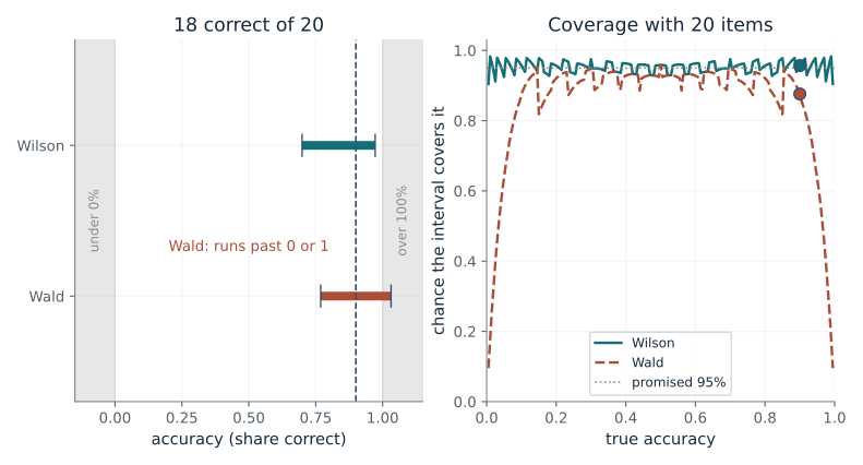
Wilson inverts a test: it keeps every true accuracy that the observed score would not reject at the stated confidence, so it never leaves [0, 1] and never collapses to a point. Wald plugs the observed accuracy into the spread, so it has no spread when accuracy is 0 or 1. The right panel counts, over every possible score, how often each interval covers the truth.

Predict first: A model gets all 10 of 10 questions right. Does the 95% Wald interval say anything useful, and how often does it capture a true accuracy of 0.98?

Number of test questions (m): 20

1010000

True accuracy

With 18 of 20 correct, Wilson gives 0.699 to 0.972 while Wald gives 0.769 to 1. If the true accuracy were 0.9, Wilson would cover it 95.7% of the time and Wald 87.6%.

Observed accuracy: 0.9
Wilson 95% interval: 0.699 to 0.972
Wald 95% interval: 0.769 to 1 (raw run past 0 or 1)
Chance Wald covers the truth: 87.6%

Why it matters for language models

Model accuracies on many benchmarks sit near the ceiling, exactly where the common formula breaks. An honest error bar on a leaderboard score needs an interval that behaves there.

Show the calculation

Wilson = (a + z^2/2m +- z sqrt(a(1-a)/m + z^2/4m^2)) / (1 + z^2/m) with a = 0.9, m = 20, z = 1.96. Wald = a +- z sqrt(a(1-a)/m) = 0.9 +- 0.131. Wald collapses to a point when a is 0 or 1 and can leave [0, 1] near the edges.

The equations and symbols

$\hat a=\frac km,\qquad \text{Wilson: }\frac{\hat a+\frac{z^2}{2m}\pm z\sqrt{\frac{\hat a(1-\hat a)}{m}+\frac{z^2}{4m^2}}}{1+\frac{z^2}{m}}$

$\text{Wald: }\hat a\pm z\sqrt{\frac{\hat a(1-\hat a)}{m}}$

m: number of test questions
k: number answered correctly
a-hat: observed accuracy, k/m
z: 1.96 for a 95% interval

Where the conclusion applies

The interval has sampling meaning only if the benchmark items are treated as a random sample from a larger target population; it is then about that population's accuracy, not the exact score of the closed benchmark. Items are independent and equally likely to be answered correctly. The control sets the true accuracy used for coverage, and k is the nearest whole number to accuracy x m. Wald numbers outside [0, 1] are impossible and are shown as clipped.

Check your understanding: A model scores 0 of 20. What does the Wald interval give, and is the Wilson lower limit 0?

Wald gives 0 to 0, a zero-width interval. The Wilson interval is about 0 to 0.161: the lower limit is 0 and the upper limit is positive, because 20 questions cannot rule out a small true accuracy.

Book source: Chapter 17, 17.2.1 Closed-World Statistics. Illustration C17-D05. Statistical identity. Book Wilson formula and worked values (m = 100, k = 90 gives about 0.83 to 0.94; m = 10,000 gives about 0.894 to 0.906). The Wald interval is the textbook comparison added here. Coverage is computed exactly from the binomial distribution, not simulated. v39 EPUB / v43 print.

06 / 08

Why a score must reward honesty

From Chapter 17, 17.9.3 Proper Scoring Rules

If a model is paid by its score, which scoring rule makes reporting its true belief the best strategy?

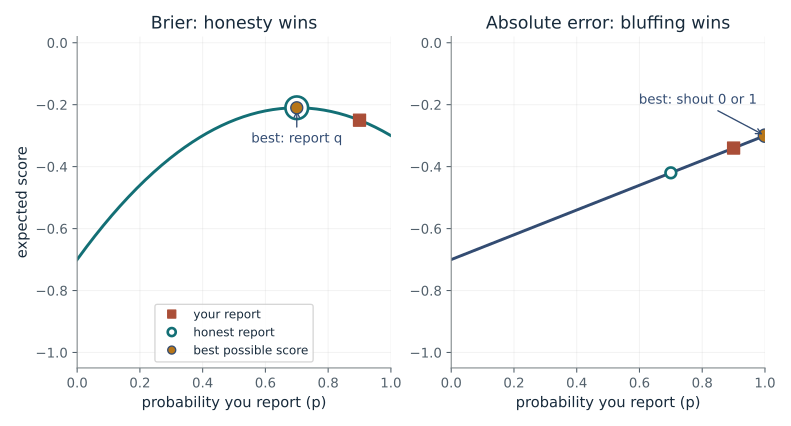
Under the Brier rule the expected score is a downward curve in the reported probability whose peak sits exactly at the true chance, so any other report loses by the squared gap. Under absolute error the expected score is a straight line, so it has no peak at the truth and the best report is an extreme.

Predict first: The true chance is 0.3. Which report earns the most expected score under the Brier rule, and under the absolute-error rule?

True chance of the outcome (q): 0.7

0.10.9

Probability you report (p)

Two curves of expected score against reported probability: Brier peaks at the true chance; absolute error is a straight line peaking at 0 or 1. — **A proper rule such as Brier makes the honest probability the best report; an improper rule rewards exaggeration.**
True chance of the outcome (q): 0.7 · Probability you report (p): 0.9

Reporting 0.9 when the true chance is 0.7 costs 0.04 in Brier score, exactly (p - q)^2. The absolute-error score changes by 0.08 and keeps rewarding a report pushed toward 1.

Brier score, honest report: -0.21
Brier score, your report: -0.25
Absolute score, honest report: -0.42
Absolute score, your report: -0.34

Why it matters for language models

If training or evaluation pays a model by a rule that is not proper, it learns to hide its real uncertainty. Brier and log loss are used for calibration because honesty is optimal under them.

Show the calculation

Expected Brier = -[q(1-p)^2 + (1-q)p^2] = -[0.7 x 0.01 + 0.3 x 0.81] = -0.25. At p = q this is -q(1-q) = -0.21; the gap is (p-q)^2 = 0.04. Expected absolute score = -[q(1-p) + (1-q)p] = -0.34, a straight line in p.

The equations and symbols

$S(p,y)=-(p-y)^2,\qquad \mathbb E_{Y\sim q}[S(p,Y)]=-q(1-p)^2-(1-q)p^2$

$\frac{d}{dp}\,\mathbb E[S]=2q-2p=0\;\Rightarrow\;p=q,\qquad \mathbb E[S(q,\cdot)]-\mathbb E[S(p,\cdot)]=(p-q)^2$

q: true chance the outcome is 1
p: probability the forecaster reports
y: the outcome, 0 or 1
S: score, higher is better

Where the conclusion applies

A single binary outcome with true chance q known to the reporter, and a reporter who maximizes expected score. The absolute-error score is improper: its expected value is a straight line in p, so the best report is 0 or 1 whenever q is not 0.5. The slider avoids q = 0.5, where that line is flat.

Check your understanding: The true chance is 0.8 and you report 0.6. How much expected Brier score do you lose against honesty?

You lose (0.6 - 0.8)^2 = 0.04. Check: honest -0.8 x 0.2 = -0.16; reported -(0.8 x 0.16 + 0.2 x 0.36) = -0.2; the difference is 0.04.

Book source: Chapter 17, 17.9.3 Proper Scoring Rules. Illustration C17-D06. Identity. Book Definition 17.8 and the Brier-score proof in the binary case. The absolute-error score -|p - y| is an added illustration of an improper rule. v39 EPUB / v43 print.

07 / 08

Easy and hard questions in one number

From Chapter 17, 17.12.2 Item Response Theory

Two models can score the same raw accuracy on a benchmark. How do item difficulty and sharpness change what each answer tells us?

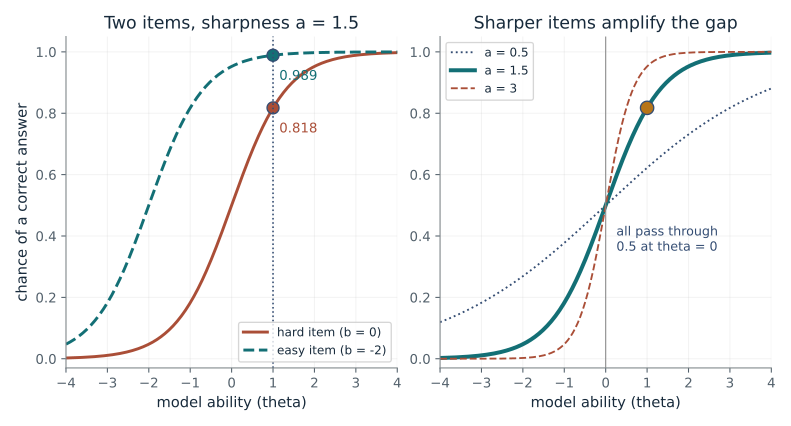
The exponent is sharpness times the gap between ability and difficulty. When ability exceeds difficulty the exponent is positive and the chance rises above one half; when it falls short the chance drops below. A larger a makes the same gap count for more. At ability equal to difficulty every a gives exactly 0.5.

Predict first: A weak model (ability -1) faces the hard item (difficulty 0). Does a sharper item (larger a) help it?

Model ability (theta): 1

-22

Item sharpness (a)

Left: success chance against ability for a hard and an easy item, model marked. Right: the hard item at three sharpness values. — **Discrimination does not make an item easier or harder: it amplifies the gap between ability and difficulty, up or down.**
Model ability (theta): 1 · Item sharpness (a): 1.5

A model of ability 1 answers the hard item with chance 0.818 and the easy one with 0.989. Ability is above the hard item's difficulty, so sharper items push its chance up.

Chance correct, hard item: 0.818
Chance correct, easy item: 0.989
Raw accuracy on both items: 0.903

Why it matters for language models

A leaderboard that averages percent-correct treats every question as equally informative. Item-response weighting shows why swapping a few highly discriminating questions can reorder models with no real change in ability.

Show the calculation

Hard item: sigma(1.5 x (1 - 0)) = sigma(1.5) = 0.818. Easy item: sigma(1.5 x (1 + 2)) = sigma(4.5) = 0.989. sigma(z) = 1/(1 + e^-z). With a = 1.5 and ability 1 the book gets 0.818 and 0.989.

The equations and symbols

$\Pr(\text{model } j \text{ correct on item } i)=\sigma\big(a_i(\theta_j-b_i)\big),\qquad \sigma(z)=\frac{1}{1+e^{-z}}$

$a=1.5,\;\theta=1,\;b=0:\quad \sigma(1.5)\approx0.818$

theta: model ability
b: item difficulty (ability at which the chance is 50%)
a: item discrimination: how sharply it separates strong from weak
sigma: logistic function mapping any number to a probability

Where the conclusion applies

A two-parameter logistic model: one ability per model, one difficulty and one discrimination per item, independent answers given those. These are parameters of a fitted model, not measured facts, and real items need not follow the logistic form. Raw accuracy on both items weights them equally.

Check your understanding: Ability 0.5, difficulty 1.5, discrimination 2. What is the chance of a correct answer?

The gap is 0.5 - 1.5 = -1, times 2 gives -2, and sigma(-2) = 1/(1 + e^2) = 0.119. The model is weaker than the item, so the chance is well below one half.

Book source: Chapter 17, 17.12.2 Item Response Theory. Illustration C17-D07. Model identity. Book Definition 17.12 and its worked examples: a = 1.5, hard item b = 0, easy item b = -2, abilities 1 and -1 (probabilities 0.818, 0.989, 0.182, 0.818). Other discriminations are illustrative. v39 EPUB / v43 print.

08 / 08

Turn scores into head-to-head win chances

From Chapter 17, 17.12.3 Bradley-Terry and Arena Rankings

If each model has one strength score, how often does a model with the higher score win a comparison?

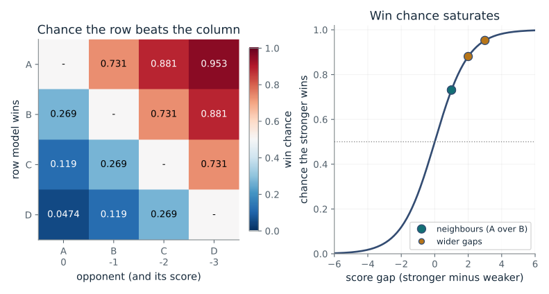
Each cell of the table is the logistic function of the row model's score minus the column model's. Equal scores give 0.5, a gap pushes the chance toward 1 without reaching it, and a cell plus its mirror cell always sums to 1. Because the table comes from differences, it can never contain a cycle.

Predict first: Neighbouring models differ by 1 score point. If the gap doubles to 2, does the stronger model's win chance double?

Score gap between neighbours: 1

05

Number of models

Left: heatmap of win chances between four models, strongest first. Right: logistic curve of win chance against score gap with the table's gaps marked. — **A score gap becomes a win probability through a logistic curve, which saturates: doubling the gap does not double the chance.**
Score gap between neighbours: 1 · Number of models: 4

Neighbouring models differ by a score gap of 1, so the stronger one wins 73.1% of the time. A over D is 95.3%: a bigger gap pushes the chance toward 1 without reaching it. Scores give win chances, not a verdict on one prompt.

A beats B: 0.731
A beats D: 0.953
D beats A: 0.0474
Score gap between neighbours: 1

Why it matters for language models

Arena-style leaderboards turn many pairwise votes into one rating per model. Reading a rating gap as a win chance needs this curve, and the single-score assumption behind it is exactly what to test.

Show the calculation

P(i beats j) = 1/(1 + e^-(s_i - s_j)). A over B: gap 1, so 1/(1 + e^-1) = 0.731. A over D: gap 3, so 0.953. Row i against column j plus row j against column i always sum to 1.

The equations and symbols

$\Pr(i\text{ beats }j)=\frac{1}{1+e^{-(s_i-s_j)}}=\sigma(s_i-s_j)$

$\Pr(i\text{ beats }j)+\Pr(j\text{ beats }i)=1$

s_i: strength score of model i
s_i - s_j: score gap between the two models
sigma: logistic function turning a gap into a win probability

Where the conclusion applies

A single strength score per model, so the model is transitive by construction: if A beats B and B beats C more than half the time, A beats C more than half the time. Real preference data can violate this (context, rater groups, length effects), and then no scores fit well. Here model A is strongest and each next model is the chosen gap below.

Check your understanding: Model X has score 3 and model Y has score 1. How often does X win, and how often does Y?

The gap is 2, so X wins sigma(2) = 1/(1 + e^-2) = 0.881 of the time and Y wins 0.119. The two chances sum to 1.

Book source: Chapter 17, 17.12.3 Bradley-Terry and Arena Rankings. Illustration C17-D08. Model identity. Book Bradley-Terry formula for pairwise win probability. The evenly spaced scores and the number of models are illustrative; no real leaderboard is reproduced. v39 EPUB / v43 print.

Estimate the mass of what has not appeared

Trade answer coverage against error and cost

Follow an answer back to usable evidence

Generate an option, then recognize it

How sure is an accuracy number?

Why a score must reward honesty

Easy and hard questions in one number

Turn scores into head-to-head win chances

Bring the idea to a question of your own