Chapter 2 , Geometry: Estimate Shape Before Measuring It
A circle’s radius grows by . Does its area grow by , , or ? The exact answer is , but the fast answer, about , may be all a design conversation needs. More important, either answer can be reached without calculating the old or new area.
That is geometry’s great economy. A diagram may invite measurement and a formula sheet may invite substitution, yet shape often reveals the answer before either begins. Similarity predicts how length, area, and volume respond to scale. Containment supplies hard ceilings. The triangle inequality rejects impossible data. Curvature, turns, coordinates, and convexity provide compact checks on calculations that would otherwise be easy to mistrust.
The twelve rules in this chapter fall into three families. The first predicts how shape responds to scale. The second establishes feasibility and bounds before exact computation. The third extracts useful information from arcs, polygons, coordinates, and mass distributions. Together they support one governing habit: estimate shape before measuring it.
Geometry is especially unforgiving of a plausible-looking number attached to an impossible figure. A one-line scale, containment, or feasibility check can prevent an exact calculation from answering a question the figure never posed.
2.1: Predict How Shape Responds to Scale
Resizing a figure does not resize all of its properties equally. The three rules in this section turn one linear scale factor into predictions about area, volume, boundary effects, and small changes in circular area.
2.1.1: Remember the square-cube laws for similar shapes
History
Scale a drawing by three and area does not triple, it grows ninefold. Book VI of Euclid’s Elements, compiled in Alexandria around 300 BCE, proved that similar plane figures compare in the duplicate ratio, the square, of their corresponding sides, and that triangles sharing an altitude scale with their bases, a plane-geometry core documented in his text. Book VI never extends the argument to solids. Carrying that same reasoning from length and area into volume, and packing all three into one rule, belongs to this book; the proportions themselves are his. One measured ratio now predicts how every other dimension of a scaled figure will move.
The equation
If every corresponding length of a geometrically similar figure is multiplied by , then
Consequently, ratios made from different dimensions acquire the corresponding difference of powers. For example, scales like .
How to read it
A length runs in one direction, area covers two, and volume fills three. Similarity multiplies every direction by the same scale factor, so length, area, or volume scale by that factor raised to the matching power. Doubling a model doubles every length, quadruples every area, and multiplies every volume by eight, the same jump a moving box makes when each side doubles: four times the floor space, eight times what it holds.
This is the geometric version of the proportional reasoning introduced in Chapter 1: identify the ratio first, then raise it to the dimension being measured. The rule predicts a ratio, not an absolute value: without one measured length, area, or volume to start from, it has nothing to multiply.
How to use it
A manufacturer builds a full-scale prototype of an engine housing after tests succeeded on a half-scale model. Every length in the full-scale part is twice the model’s, so . Quantities built from area, like the sheet metal in the housing’s skin, rise by ; quantities built from volume, like the metal cast into a solid mounting bracket, rise by . A bracket that used 0.5 kilograms in the model needs close to kilograms full scale, not the kilogram a simple doubling would suggest.
The estimate assumes a faithful enlargement. If the production version hollows out the bracket, thins a wall that stayed fixed in the model, or switches to a denser alloy, material use departs from the cube law and must be recalculated directly. This is an Independent rule: when similarity holds, it directly predicts the new geometric quantity across many applications.
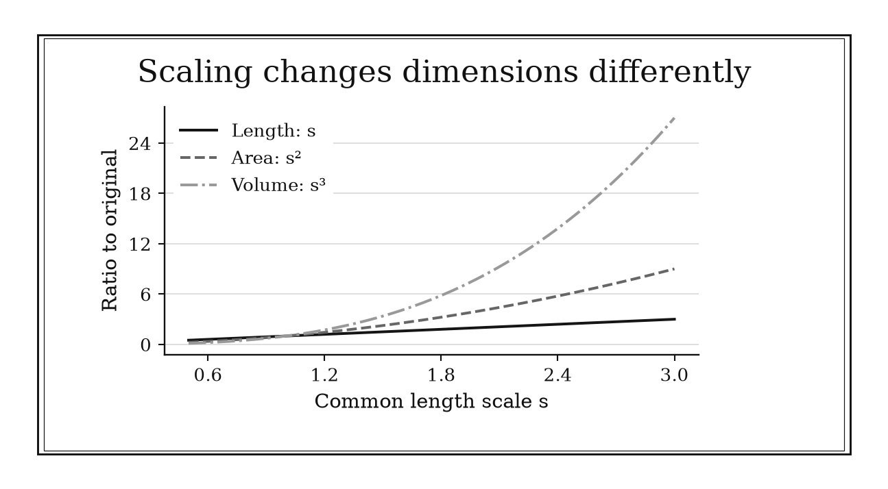
Figure 2.1. For similar shapes, doubling every length multiplies area by four and volume by eight. These are geometric ratios; changes in shape or material require a different calculation.
2.1.2: Expect boundary-to-area ratio to shrink like inverse size
History
Why can’t a giant simply be a scaled-up man? Galileo took the question seriously in Two New Sciences, published in Leiden in 1638. Comparing geometrically similar structures and animals, he argued that an animal or a beam enlarged faithfully does not keep its mechanical proportions: cross-sections and bulk grow at different rates, so the large copy is not a bigger version of the small one but a structurally different object. That mismatch of scaling powers is the engine of this rule. Writing it as a boundary-to-area ratio is a modern shorthand, not Galileo’s phrasing, but the observation is his: size alone changes how much boundary serves each unit of interior.
The equation
For a planar figure scaled by ,
and therefore
The three-dimensional companion is .
How to read it
Here is the distance around a shape (its perimeter) and is the area inside. The rule says that when you enlarge a shape without changing its proportions, boundary per unit of area drops by exactly the enlargement factor. Both quantities still grow; the edge just grows slower. Doubling a figure multiplies its edge by 2 but its interior by 4, so each unit of interior gets by with half the boundary. A kitchen version: a dinner roll is mostly crust, while a large loaf from the same recipe is mostly crumb. The rule compares a shape with an enlarged copy of itself. It says nothing about two different shapes: a ribbon and a square of equal area have very different perimeters.
How to use it
A community garden committee runs a square plot 10 meters on a side and is voting on a move to a 20 meter square. The treasurer wants a fast read before pricing anything. Growing space follows area: square meters becomes , four times the beds. Fencing follows the boundary: meters becomes , only twice the fence. Fence per square meter of garden falls from to , exactly the halving that predicts for . Enclosure gets cheaper per bed at the larger size, so the treasurer endorses the move and budgets fencing at double, not quadruple, the current bill. The catch sits in the similarity requirement. If the new land is a long strip along a road, or four scattered plots, boundary does not thin out; scattered or elongated pieces can demand more fence per unit of area than the little square did. Check that the new shape is really a scaled copy before trusting the ratio. This is an Independent rule: under similarity, it directly predicts how a broad class of boundary effects changes with size.
2.1.3: Double the fractional radius change to estimate circle-area change
History
A small error in a circle’s radius does not stay small in its area: it roughly doubles. Archimedes confronted a related problem around 250 BCE in Syracuse, hunting a guaranteed interval around the circle’s true measure. In Measurement of a Circle, he bounded the circumference by repeatedly doubling the sides of inscribed and circumscribed polygons, reaching 96 sides and tying the curve to computable chords with explicit bounds. He never wrote the differential shortcut below; reading a small fractional radius change as doubling into a fractional area change is a later local reading of the exact area law his bounds surround. His bounds endure in the rule below as a way to know how far a small change moves the answer.
The equation
Let and write the fractional radius change as
Then the exact fractional area change is
When ,
How to read it
Radius appears twice in , so a small percentage change in radius produces about twice that percentage change in area: a 1% larger radius gives roughly 2% more area. The part left out is the change squared, so small for modest changes it barely registers, like the last puff of air that tops off a bicycle tire already near full pressure. For a growing radius the true increase is a touch more than double; for a shrinking radius the true decrease is a touch less severe than double predicts, since the dropped term is always positive.
The shortcut does not distinguish diameter from radius: a fractional change in diameter is the same fractional change in radius, so double it only once. It also stops being trustworthy once the change itself is large.
How to use it
A pizzeria is deciding whether to advertise its 14-inch pizza as roughly double a personal 10-inch pie. The radii are 7 and 5 inches, a increase, so the estimate predicts , about 80% more area. The dropped correction is , so the exact increase is , not : too far off to trust for pricing dough by the ounce, so the kitchen uses the exact squared ratio instead.
For a smaller adjustment the shortcut holds up well. Moving a pan from a 9-inch to a 9.5-inch radius is an increase of , predicting , about 11% more area; the dropped correction is , close enough for adjusting dough weight without recalculating the exact area. The dividing line is the size of the change itself. This is an Independent rule: it produces a direct sensitivity estimate wherever circular area depends on a changing radius.
2.2: Bound First, Compute Second
A bound can be more useful than a decimal. The three rules in this section reject impossible triangles, place hard ceilings on complicated regions, and fence in a diagonal before a square root is evaluated.
2.2.1: Check the triangle inequality before doing triangle algebra
History
Feed three impossible lengths into Heron’s formula and the arithmetic collapses into the square root of a negative number, an error that appears only afterward. Around 300 BCE in Alexandria, Euclid had closed that door in Book I of the Elements: Proposition 20 proved that any two sides of a triangle together exceed the third, and Proposition 47, in the same book, fixed the squared relation between a right triangle’s legs and hypotenuse. Both results are explicit in his text. Euclid’s proposition stops at proving the inequality. Turning it into an instant pass-or-fail gate before Heron’s formula or a construction drawing is this book’s workflow addition; the test catches bad data before a longer calculation dresses it up as a real triangle.
The equation
For proposed side lengths sorted so that
a nondegenerate Euclidean triangle requires
If , the points are collinear and the area is zero. If , no such triangle exists.
How to read it
The straight segment joining two points is the shortest path between them, the way a delivery route can never beat a straight line home no matter which streets it takes. Traveling along the remaining two sides of a proposed triangle must therefore be longer than the direct side. Once the three lengths are sorted smallest to largest, only the largest needs checking: the other two inequalities follow automatically once every length is positive.
This rule answers feasibility, not shape. Passing the test does not say whether the triangle is acute, right, or obtuse, and it does not determine its area.
How to use it
A carpenter framing a triangular roof truss receives cut lengths of 4, 7, and 12 feet for the three members. Sorted and tested, : the pieces cannot close into a triangle at all, so before nailing anything the carpenter flags the delivery, since one length was almost certainly cut wrong.
A replacement piece arrives at 10.9 feet instead of 12. Now , feasible, but the margin is only feet. If each board is measured to the nearest tenth of a foot, that margin sits inside the measurement error itself, so feasibility is not solid enough to declare without the tolerance on every cut. A truss this close to degenerate is also nearly flat, amplifying small board errors into large roof-pitch errors.
Run this check before cutting, welding, or bracing, and keep all lengths in the same unit. This is an Independent rule: it directly answers whether a nondegenerate triangle can exist, even when a larger calculation would have followed.
2.2.2: Use a bounding box for a fast area or volume ceiling
History
A rectangle drawn around a complicated shape gives an instant ceiling, a shortcut surveyors, packers, and graphics programmers reach for by habit. Nobody can name the day that reflex became a rule. Rectangular enclosures appear constantly in surveying and packing, but the search behind this book found no dated episode where this exact ceiling was the documented, decisive calculation; an old drawing of a shape inside a rectangle illustrates containment, not this rule’s history. A name or priority claim alone would not show how the bound settled a real question. Closing this evidence gap would take a dated calculation or institutional record where the bound itself changed a decision. Until then, this reads as folk mathematics, a containment idea so obvious it spread through practice, not a paper trail.
The equation
If a planar region is contained in a rectangle of width and height , then
If a three-dimensional body is contained in a rectangular box with side lengths , then
How to read it
Area and volume are monotone under containment: a shape can never occupy more space than a box built to surround it, the same way a moving box has to be at least as large as everything crammed inside. The box only remembers a shape’s extreme edges and throws away every notch and curve in between. That loss of detail makes the bound instant, and loose.
The result is a ceiling, not an estimate of typical size. It can prove a reported answer is too large to be true. It cannot certify that a smaller reported answer is correct.
How to use it
An environmental surveyor is checking a consultant’s report on an irregular lake spanning 8 kilometers east to west and 5 kilometers north to south. Whatever the shoreline’s coves and inlets, its surface area cannot exceed square kilometers. The report claims 53: impossible under those coordinates, rejected before checking a single meander of shoreline. A second claim of 27 passes the check, though the box alone cannot confirm it is accurate.
The same idea covers a park’s fill volume, and pairing the box with a known inner shape tightens it into a bracket. If the parcel runs diagonally across the surveyed grid, the axis-aligned box can enclose mostly empty land, so rotating the box or splitting the parcel gives a tighter check when the stakes justify the work. Confirm every extreme coordinate belongs to the same survey before trusting the ceiling. This is an Independent rule: it supplies a hard plausibility limit across many geometric and physical calculations despite the unresolved historical episode.
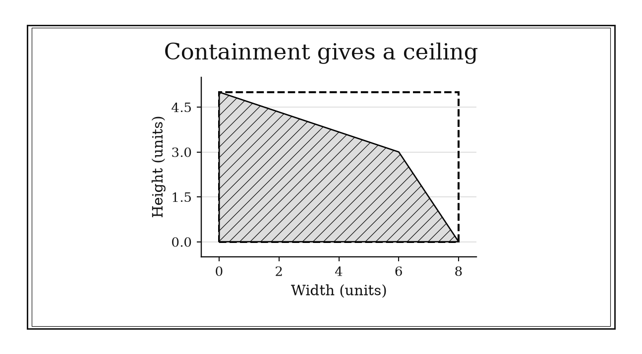
Figure 2.2. This constructed 8-by-5 bounding rectangle has area 40. The shaded polygon occupies 27 square units. Containment rules out 53, but cannot by itself certify a claim of 27.
2.2.3: Bracket a right-triangle diagonal before taking a square root
History
A rectangular diagonal cannot be found without a square root, but its plausible range can be fenced in before that root is ever computed. Euclid supplied both fence posts in Book I of the Elements. Proposition 47 gives the squared relation between a right triangle’s legs and hypotenuse; Proposition 20, in the same book, establishes that any two sides of a triangle exceed the third. Together the theorems constrain a diagonal before its exact value is worked out. Euclid never packaged the propositions as the bracket used below; the ancient theorems are his, and using them as a rapid calculator check and transcription guard is this book’s reading of what they jointly imply. Their combined payoff is a safety net around every diagonal calculation that follows.
The equation
For component lengths and Euclidean diagonal
we have
When , both inequalities are strict.
How to read it
The diagonal cannot be shorter than either perpendicular component, the way a route across a rectangular lot can never be shorter than the straight distance along just one side: dropping one nonnegative square from the sum gives that lower bound. Nor can it be as long as walking the two legs one after another, since squaring the upper candidate adds the positive term :
The bracket is deliberately cheap: a safe interval, not a close approximation for every shape of rectangle. The lower bound is nearly exact when one leg is tiny beside the other; the upper bound is approached only as one leg shrinks toward zero.
How to use it
A logistics crew needs to run a cable diagonally across a warehouse floor measuring 9 by 12 meters. Before pulling cable or trusting a supplier’s spec sheet, the bracket gives . The exact length is meters, comfortably inside the interval, so the crew orders 15 meters with confidence. A cut sheet listing 25 meters or 10.5 meters would be rejected on sight, no square root required.
For a long, narrow conduit run of 1 by 100 meters, the lower bound of 100 is almost the whole answer; the bracket earns its keep fastest on elongated runs like this. On a nearly square room the interval is wide and far less decisive, so the crew should not skip the exact calculation just because the bracket passed. Sort the legs, convert both to the same unit, and write the interval before ordering material. This is an Independent rule: it directly bounds a distance across many settings before or after exact evaluation.
2.3: Extract Information from Curves and Coordinates
Curves and coordinate lists often hide simple structure. The six rules in this section turn a shallow arc into a length estimate, a full turn into polygon angles, coordinates into area, and positive weights into a location check.
2.3.1: Estimate shallow-arc sagitta by chord squared over radius
History
A 96-sided polygon squeezed between a circle’s inscribed and circumscribed edges is the physical image behind this rule. Around 250 BCE in Syracuse, Archimedes built exactly that figure in Measurement of a Circle, doubling the sides of inscribed and circumscribed polygons until the circle’s curvature was trapped between two computable chord lengths. Archimedes never wrote the shallow-arc sagitta formula below. The rise of a short arc above its chord, read as chord squared over eight times the radius, belongs to the same chord geometry his polygons made possible. His method bought a way to replace a curve with straight lines close enough to trust.
The equation
For a chord of length in a circle of radius , the minor-arc sagitta is
Rationalizing gives the exact stable form
When ,
How to read it
The sagitta is how far the middle of a short arc bulges above its straight chord, the bow’s rise above its string. For a shallow arc, the bulge is close to chord length squared divided by eight times the radius: curvature grows with the square of the span and shrinks in direct proportion to the radius. Doubling a short chord makes the bulge about four times as large; doubling the radius while holding the chord fixed makes it about half as large.
Expanding one term further gives
so the shortcut runs slightly low, harmless for a shallow arc, worse as the arc deepens. As with nearby square roots in Chapter 1, rationalizing the exact expression first separates a stable rewrite from the approximation built on it.
How to use it
A civic inspector is checking whether a long, gently curved pedestrian bridge deck has developed sag. The deck’s design radius is 500 meters, and the inspector measures a 10-meter chord across the walkway. The predicted sagitta is meters, or centimeters of expected rise. The ratio is small, so the shallow-arc estimate is trustworthy at this scale; the exact formula gives essentially the same 2.5 centimeters.
A measured 3-centimeter rise instead of 2.5 is a real deviation worth flagging, not an approximation artifact. The estimate would mislead on a sharply curved arch rather than a gentle deck: once the chord spans a large fraction of the radius, the shortcut runs low and the exact formula must be used instead. Confirm the chord is well under the radius before trusting the shortcut. This is an Independent rule: it directly converts radius and span into a broadly useful curvature estimate.
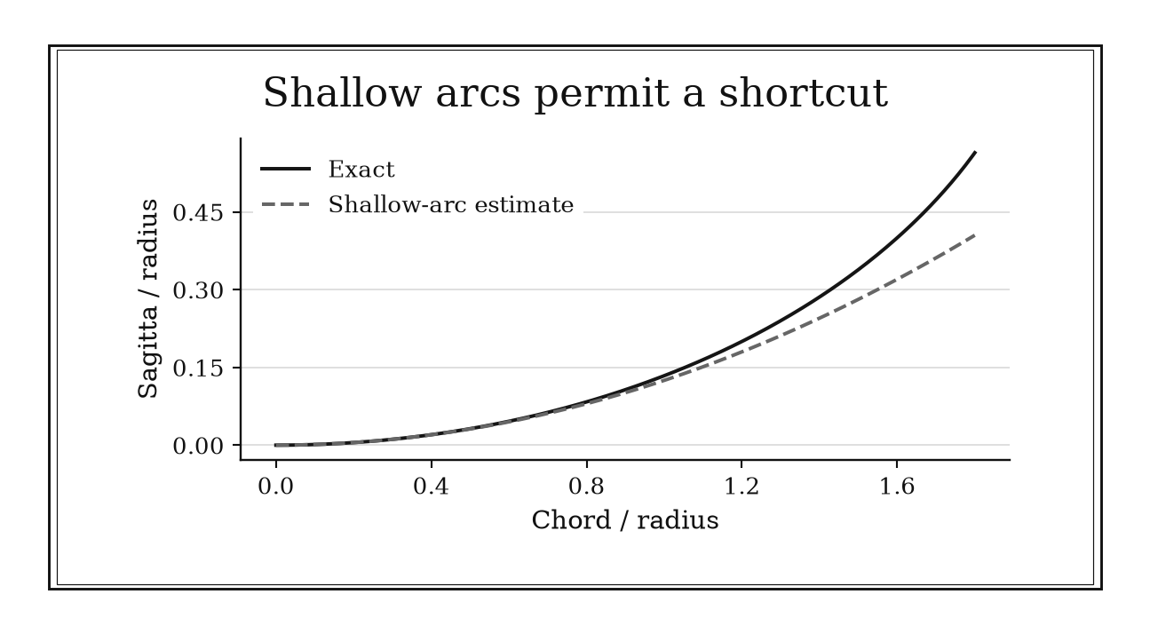
Figure 2.3. With u=L/R, the exact minor-arc rise is s/R=1-sqrt(1-u²/4). The approximation u²/8 runs low and becomes less reliable as the chord grows relative to the radius.
2.3.2: Estimate regular-polygon angles from the exterior turn
History
A picture frame built on the wrong angle assumption will not close, and every joint will show the gap. Euclid’s Book I, Proposition 32, guards against exactly that: he proved the triangle angle sum and the straight-line angle relations that let any polygon be cut from one vertex into triangles. A convex -sided figure splits into triangles this way. Euclid proved the underlying angle sum; dividing one full turn by for a regular polygon packages that triangulation into a shortcut his own text never states. The payoff is a fast check on any polygon a builder intends to close.
The equation
For a regular -gon,
and
Equivalently, the sum of the interior angles of a simple -gon is .
How to read it
Walk once around the outside of a convex polygon, like tracing a picture frame with your finger, and your direction turns through one full revolution, . Regularity makes all turns equal, so each receives . At a vertex, the interior angle and its exterior turn form a straight line and add to .
As grows, each turn shrinks toward zero and each interior angle creeps toward , which is why a many-sided regular polygon looks locally almost straight.
For any simple -gon, regular or not, is only the average interior angle. Regularity is what promotes that average to the actual value at every vertex; keeping the two statements separate prevents a sum formula from being misapplied as a local-angle formula.
How to use it
A woodworker building a regular twelve-sided picture frame needs the miter angle for each joint. With , the exterior turn is , so the interior angle is ; each piece is mitered at half that turn, off square, the standard shop convention for regular-polygon frames. A quick check confirms the plan: twelve interior angles of total , matching .
The relation also runs in reverse: a jig set to turn at every joint yields sides, not twelve, catching a jig-setting mistake before the first cut. The shortcut assumes the frame is meant to be regular: an irregular hexagonal frame will still have exterior turns summing to , but no single turn applies to every corner, and forcing one will leave a gap at the last joint. Keep degrees and radians straight, since one full turn is radians. This is an Independent rule: symmetry and a full turn directly determine the angles in any regular polygon.
2.3.3: Expect regular-polygon circle error to fall quadratically
History
How many sides is enough? A polygon approximation never reaches its circle; the gap only shrinks on a predictable schedule as the count climbs. Archimedes pushed that refinement hard: around 250 BCE in Syracuse, in Measurement of a Circle, he bounded the circumference between inscribed and circumscribed regular polygons, doubling the side count repeatedly until, at 96 sides, the bounds were tight enough to constrain sharply. That use of polygons and bounds is documented fact. The precise law that the leading error falls in proportion to comes from a modern small-angle expansion, not a convergence analysis Archimedes himself stated. What his doubling demonstrated in practice, the modern law now predicts in advance.
The equation
The perimeter of a regular -gon inscribed in a circle of radius is
Using gives
Thus the leading relative perimeter deficit is approximately .
How to read it
The inscribed perimeter falls short because every straight chord cuts inside its arc, never along it. That shortfall shrinks in proportion to , similar to a photo that sharpens less with each doubling of resolution. Doubling the number of sides multiplies the leading error by
roughly two bits of accuracy each time. This is a statement about the rate of convergence: it does not promise the current error is small, only that a further doubling cuts whatever remains by about three quarters.
Reducing the leading error by a factor of requires multiplying by about : times as many sides gives about a hundredth the error, turning “use more segments” into a budget. For a unit circle, and against : the deficits are and , the second about one quarter of the first.
How to use it
A machinist programming a CNC router to cut a circular part approximates the circle with an inscribed 20-sided polygon path. The leading relative deficit is : the toolpath’s perimeter runs about that much short of the true circumference. Doubling the toolpath to 40 sides predicts a shortfall of , one quarter as large, without a new trigonometric calculation.
If the part’s tolerance calls for under deviation in perimeter, the shop can commit to 40 sides in advance and expect it to clear the spec, instead of cutting and measuring a test part. The forecast assumes the toolpath stays a regular inscribed polygon at reasonably large : a coarse 6-sided approximation, an irregular CAM export, or an error dominated by tool deflection rather than geometry will not follow the same quartering pattern. This is an Independent rule: it directly forecasts refinement payoff for an important family of geometric approximations.
2.3.4: Use the shoelace formula for polygon area from coordinates
History
Every surveyor’s manual teaches the shoelace method; nobody can point to the day it was tied. The coordinate-area formula is often traced through an attribution chain running from Carl Friedrich Gauss to A. L. F. Meister, but the accounts inspected for this book disagree about priority and about how the classroom name spread from either one. Without a directly inspected primary publication containing the operative formula, no dated origin event clears this book’s evidence bar, leaving an evidence gap. Closing it would need a located primary text, in Gauss’s, Meister’s, or another hand, stating the cross-multiplication rule and dated with confidence. Until such a text surfaces, the fairest description is folk mathematics: a crisscross bookkeeping trick that spread through practice long before anyone wrote down where it came from.
The equation
For vertices listed in cyclic order, with ,
Before taking the absolute value, the sum gives twice the signed area.
How to read it
Each pair of neighboring corners, read in order around the boundary, contributes a small signed triangle area measured back to a fixed origin point, the way a delivery zone can be built up triangle by triangle from a single reference point. Add all those contributions and the overlapping middle pieces cancel, leaving just the plot’s own boundary contribution. Walk the corners backward and the total flips sign but not size; the formula does not care where the origin sits.
The name “shoelace” just describes the crisscross multiplication pattern in a coordinate table, lace over lace. What makes the formula valid is that the corners are listed in genuine boundary order; a scrambled list of the same points will not give the plot’s real area.
How to use it
A land surveyor receives four corner coordinates for an odd-shaped residential lot, , , , and , in tens of meters, listed in walking order. Cross-multiplying neighboring pairs and summing gives forward and reverse, so the signed area is , or square meters, the figure that goes on the deed.
Before filing that number, the surveyor checks it against the bounding-box ceiling from earlier in this chapter: the lot spans 4 by 3 units, so area cannot exceed , or square meters, and 8.5 comfortably passes. If the field crew had recorded the corners out of order, the same arithmetic would return a wrong number with no error message to flag it. Always repeat the first corner at the end of the list and never feed it an unordered point cloud. This is an Independent rule: ordered coordinates directly yield area in many applications despite the unresolved priority story.
2.3.5: Prefer base times perpendicular height when height is available
History
Three known side lengths force a slow detour through Heron’s formula and a square root; a base and its perpendicular height skip the detour completely. That shortcut rests on Book VI of Euclid’s Elements: triangles and parallelograms sharing an altitude have areas proportional to their bases. That relationship is Euclid’s own. Choosing over Heron’s formula whenever a trustworthy perpendicular height is already in hand is a method-selection habit built on his proportion; the preference itself belongs to later practice. No semiperimeter, square root, or reconstruction from three sides is needed once a base and its true height are known.
The equation
For any triangle with base length and corresponding perpendicular height ,
The altitude may meet the base segment or its extension; is the nonnegative perpendicular distance to the base line.
How to read it
Two congruent copies of the same triangle, flipped and joined, form a parallelogram with the same base and height , the way two identical wedge-shaped roof trusses fit together into a rectangle-like shape. That parallelogram has area , so one triangle is exactly half of it. Slant does not matter: sliding the top vertex sideways, parallel to the base, leaves both and unchanged.
The word doing the work is “perpendicular.” A side that merely touches the base is not automatically its height; height is measured straight up from the base line, at a right angle to it. A complicated shape can be split into triangles sharing a convenient base or height, and their areas added.
How to use it
A landscaper is pricing mulch for a triangular flower bed cut into a lawn corner, with a base along the walkway measuring 13 feet and a perpendicular depth of 6 feet. The bed’s area is immediately square feet, whether the deepest point sits directly across from the walkway, off to one side, or past the far edge of the base extended. No semiperimeter or square root is needed.
The shortcut only works if the 6-foot measurement is truly perpendicular to the walkway edge. If the landscaper instead measures along a slanted side fence, using that length as the height will overstate the bed’s true area. When only three side lengths are available, Heron’s formula remains the right tool, after checking the triangle inequality first. This is a Workflow rule: it selects the simplest area procedure when the right information is present, and it transfers across many larger geometric calculations.
2.3.6: Use the convex hull as a centroid sanity check
History
Get a center of gravity wrong and a lever, scale, or structure built on that point will not balance the way theory predicts. Archimedes confronted that stake around 250 BCE in Syracuse, opening On the Equilibrium of Planes with axioms about balance and deriving centers of gravity for plane figures from them. His arguments combine pieces of a figure by weighted positions, keeping the balance point consistent with how mass is distributed. Archimedes reasoned directly about physical centers of gravity; describing a positive weighted average as a point trapped inside a convex hull is a modern vector restatement of that constraint, not a phrase from his own text. A modern check confirms that placement in seconds; Archimedes had only his axioms to derive it.
The equation
For points carrying nonnegative weights , with total weight ,
Therefore lies in the convex hull of the contributing points.
How to read it
Nonnegative weights that add to one describe interpolation, never extrapolation, the way a marble resting on a stretched sheet between several pegs can only settle somewhere among them, never beyond. With two points, the weighted average lands on the segment joining them. Add more points and the reachable region fills out to their convex hull, the smallest convex shape containing them all. A computed centroid with genuinely positive weights that falls outside that hull flags a sign, coordinate, or weighting error upstream.
This check only narrows a permissible region. It does not pin down the centroid’s exact value, and it cannot certify that an answer sitting inside the hull is correct. The same idea covers a continuous object with nonnegative density.
How to use it
A CAD designer runs a quick balance check on a bracket modeled as three equal point masses at its mounting holes, at , , and in centimeters. The software reports a centroid of . Plotting the holes as a triangle, sits visibly inside it, so the result passes and the designer moves on.
A faulty software revision reports a centroid of for the same three holes and equal masses, outside that triangular hull, an immediate signal that a sign got flipped or a coordinate mistyped. The check assumes the point masses are genuinely positive; a negative weight for a cutout, or a subtracted region, can legitimately place the algebraic result outside the hull, so those signed pieces must be combined into one true nonnegative distribution first. This is a Workflow rule: it is a reusable audit inside centroid and averaging calculations rather than a complete method for finding every centroid.
Chapter Synthesis: A Geometric First Pass
The rules in this chapter do not form one universal measurement procedure. They form a sequence of questions that can be asked before exact measurement begins.
Start with scale. If two objects are similar, one linear ratio predicts every corresponding length, area, and volume ratio. It also reveals why boundary effects weaken relative to interior capacity and why a small radius change has twice the first-order effect on circular area.
Next establish possibility and range. Check whether proposed sides can form a triangle. Enclose a complicated region to obtain a hard ceiling. Place a diagonal between a component length and the sum of the components. These checks can reject an answer without reproducing the calculation that generated it.
Finally, choose the representation that exposes the shape: rationalize a shallow arc, read polygon angles as turns, forecast refinement through an error law, order coordinate vertices for shoelace, select base-height data when available, and use convexity to audit weighted locations.
The deeper habit is to separate four questions:
- What changes under scaling, and by which power?
- What must be true before this figure can exist?
- What containment, symmetry, or convexity bound must the answer respect?
- Does the rule answer the question directly, or choose and check a later procedure?
Most geometry rules here are independent because shape itself supplies the answer. The base-height preference and convex-hull check are workflow rules: they guide or audit a broader calculation.
One-Page Geometry Toolkit
| Recognition cue | Rule to try | What it gives | Role |
|---|---|---|---|
| Geometrically similar copies | Apply the square-cube laws | Length, area, and volume ratios | Independent |
| Boundary effect versus interior capacity | Divide the old ratio by the scale factor | New boundary-to-area ratio | Independent |
| Small fractional radius change | Double it and inspect the squared correction | Circle-area sensitivity | Independent |
| Three proposed side lengths | Compare the largest with the other two combined | Triangle feasibility | Independent |
| Complicated contained region | Multiply box dimensions | Hard area or volume ceiling | Independent |
| Euclidean diagonal or vector magnitude | Bracket between max and sum | Fast distance interval | Independent |
| Short chord on a large circle | Use | Shallow sagitta estimate | Independent |
| Regular polygon | Divide one full turn by | Exterior and interior angles | Independent |
| Refined inscribed regular polygon | Expect error proportional to | Refinement payoff | Independent |
| Cyclic coordinate vertices | Apply the shoelace cross-sum | Polygon area | Independent |
| Triangle with known perpendicular height | Use | Simplest exact area route | Workflow |
| Positive weighted points or mass | Check the convex hull | Centroid plausibility | Workflow guardrail |
Decision Path
- Are two figures scaled copies? Find the linear factor first. Raise it to the second power for area and the third for volume; subtract powers when forming ratios such as perimeter over area.
- Is the change small? Express it as a dimensionless fraction. For circle area, double the fractional radius change and compare its square with the required accuracy.
- Could the data be impossible? Test the triangle inequality before any three-side formula and check units before interpreting coordinates or lengths.
- Do you need only a plausibility range? Enclose the shape in a box or bracket a Euclidean diagonal before performing the exact computation.
- Is the boundary circular or polygonal? Use chord-radius geometry for shallow sagitta, a full turn for regular-polygon angles, and the law to predict the effect of refinement.
- Is area encoded in coordinates? Keep vertices in cyclic order and use shoelace. If a perpendicular height is already known, is usually the shorter route.
- Is the result a weighted location? With nonnegative weights, require the centroid to remain inside the convex hull.
Transfer Problems
1. Scale without rebuilding
A cylindrical storage tank is enlarged geometrically so that every length is times the original. Predict the factors by which its surface area, volume, and surface-area-to-volume ratio change. Then state one design change that would invalidate the direct prediction.
2. Reject, bound, then calculate
A survey record describes a triangular parcel with sides , , and . Decide whether it can exist. A second irregular parcel spans meters east-west and meters north-south. Give a hard area ceiling and explain what a reported area of square meters would imply.
3. Use two independent checks
The vertices , , , and are listed in boundary order. Compute their area with the shoelace formula, check it against a bounding rectangle, and determine whether the average of the four vertices must lie inside their convex hull.
Where These Ideas Reappear
- Trigonometry: shallow chords and polygon error become small-angle approximations for sine and cosine.
- Calculus: the circle-area and sagitta rules become linearization with explicit higher-order corrections.
- Analysis and asymptotics: the polygon law becomes a general question about convergence rates and leading errors.
- Applied mathematics: square-cube scaling becomes dimensional analysis, nondimensionalization, and regime comparison.
- Linear algebra: shoelace is a determinant calculation, while centroids are convex combinations and barycentric coordinates.
- Numerical methods: bounding boxes, independent brackets, and refinement ratios become standard validation and error-control tools.
- Measurement and uncertainty: near-degenerate triangles and small geometric tolerances require uncertainty to be propagated before a binary conclusion is trusted.
Historical Notes and Sources
Sources for the historical accounts in this chapter follow. The two evidence-gap entries support their mathematics without claiming an unverified origin event.
- Euclid on similarity and area: Clark University edition of Book VI and Proposition VI.1.
- Galileo on unequal scaling powers: Open Library scan of Dialogues Concerning Two New Sciences and MacTutor biography of Galileo.
- Archimedes on circle measurement: Cambridge edition record for Measurement of a Circle and Library of Congress manuscript resource.
- Euclid on triangle bounds and right triangles: Proposition I.20 and Proposition I.47.
- Euclid on triangle angle sum: Proposition I.32 and the Elements table of contents.
- Archimedes on centers of gravity: Archimedes Palimpsest project and Harvard translations and study materials.
- Modern circle-error mathematics: NIST Digital Library of Mathematical Functions, §4.19 and OpenStax on circles.
- Evidence-gap mathematics: OpenStax on plane area, OpenStax on volume, and MIT OpenCourseWare on the shoelace formula. These establish the calculations, not exact historical origin events for the two gap profiles.