Chapter 3: Trigonometry: Control Angles, Directions, and Oscillations
A calculator is asked for the direction of the vector . If we divide the components first, then compute
the principal answer is . But the vector points northwest, at . The division erased a half-turn before the inverse function ever saw the problem.
That failure captures a central danger in trigonometry. The arithmetic is often easy; preserving the geometry is not. An angle may be in the wrong unit, an inverse function may return only one branch, a large input may hide a familiar reference angle, or the subtraction of two nearly equal values may destroy the quantity we wanted to measure.
The ten rules in this chapter fall into three families. The first uses small angles as local models while keeping their error visible. The second protects direction, phase, and periodicity. The third solves triangles without losing branches or numerical precision. Together they support one governing habit: keep the circular structure intact while simplifying the calculation.
3.1: Use Small Angles as Local Linear Models
Near zero, the circle begins to look like its tangent line. Sine and tangent therefore resemble the angle itself, while cosine departs from one more slowly, at quadratic scale. These statements are powerful only when the angle is measured in radians and the first neglected term is small enough for the decision at hand.
3.1.1: Replace sine by the angle at small scale
History
A pendulum clock is this rule’s artifact. Christiaan Huygens built his against a stubborn defect: a real pendulum’s period changes with how wide it swings, so a clock trusted at a narrow arc drifts once nudged into a wider one. His 1673 Horologium Oscillatorium describes that fight and his cycloidal-cheek remedy, a shaped guide forcing every swing to the same period, a mechanical fix rather than a bet on the small-swing approximation holding. The sources document the clock and the cycloidal fix, the mechanical answer he trusted over any approximation. This rule keeps only the narrow-swing behavior his clock exploited: sine tracking the angle near zero, close enough to trust before it drifts.
The equation
For measured in radians,
Thus
with leading absolute error about and, for nonzero small , relative error about .
How to read it
At the origin, sine has value zero and slope one, so its tangent line is : for a small angle, sine and the angle nearly coincide. The first departure from that line is cubic, so halving a small angle cuts the leading absolute error by roughly a factor of eight and the relative error (the miss as a share of the true value) by roughly a factor of four. A tenth of a radian, about six degrees, a tilt too shallow to notice by eye, already gives absolute agreement to a few parts in ten thousand; the relative error is nearer seventeen parts in ten thousand.
Radians are part of the formula, not a formatting preference: they give sine unit slope at zero. Rule 3.3.3 makes that unit choice explicit. The rule does not say how large an angle your task can tolerate; that boundary comes from your own accuracy requirement.
How to use it
A calibration engineer on an assembly line finds a robotic arm’s angle sensor reporting a tilt of radian at the end of its -meter reach, and needs a fast estimate of tool-tip drift before ordering a recalibration. Lateral deflection is , so
The first correction is
well under the shop’s one-millimeter tolerance, so m is trustworthy. She flags the arm for a sensor reset rather than a hardware swap.
The shortcut misleads if the sensor’s raw reading is actually degrees, not radians: treating as rad overstates the drift by a factor near , since rad gives m, not m. Confirm the unit before trusting the estimate. This is an Independent rule: once the angle and tolerance pass the smallness check, it directly supplies a useful estimate in many applications.
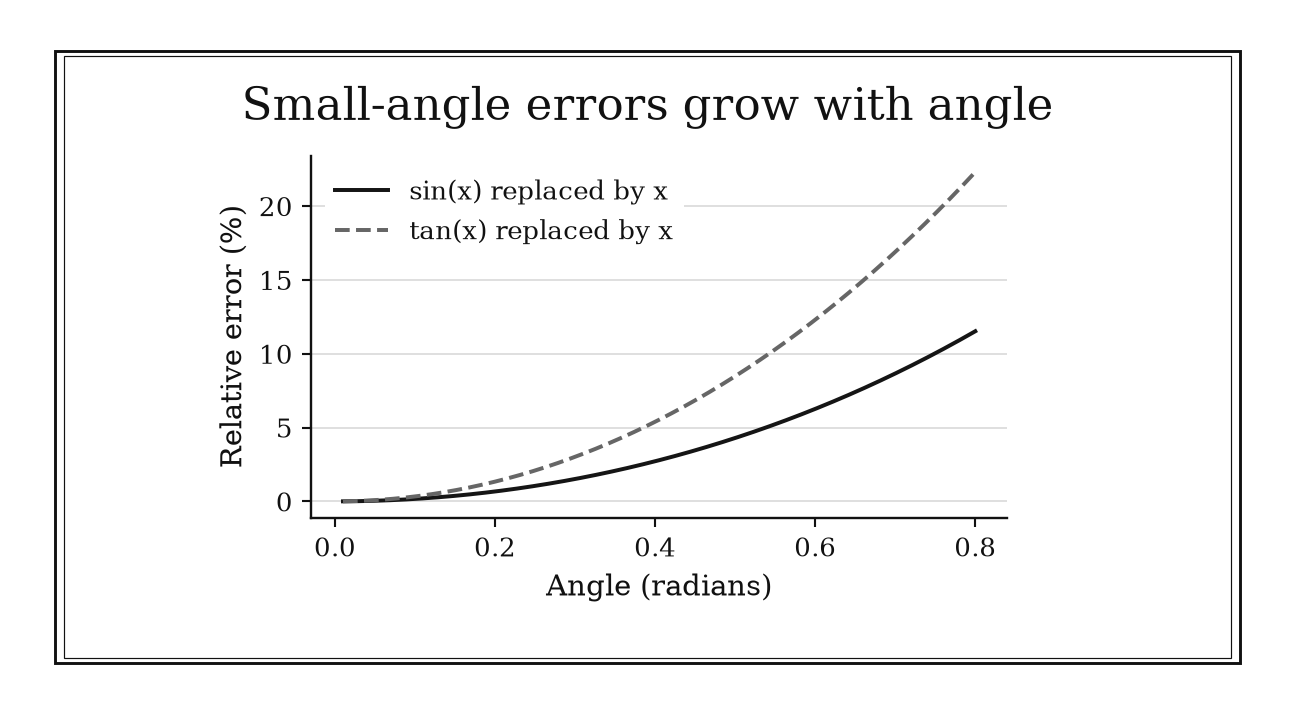
Figure 3.1. Replacing sine or tangent by the angle incurs increasing relative error. Angles are in radians; the tangent approximation departs faster over this range, which stays away from its pole.
3.1.2: Keep the quadratic correction for cosine near zero
History
Losing the small deficit here erases the entire effect under study. Huygens’s 1673 Horologium Oscillatorium describes his pendulum-clock troubles: near the bottom of a swing, a pendulum’s height above rest changes very little at first even though the swing angle grows steadily. Treat cosine as flatly equal to one there and that early height change vanishes on paper, along with the period-amplitude coupling his cycloidal cheeks were built to fix. His clock and his isochronism remedy are the documented record; crediting that early flatness to cosine’s own shape near zero is a modern reading this book adds, not arithmetic Huygens wrote himself.
The equation
For a radian angle near zero,
The useful first correction is
If this quadratic approximation is used, the leading omitted term has size about .
How to read it
Cosine is even, unchanged when flips sign, and its slope at zero is also zero. There is no linear term, so the first loss from the maximum value is quadratic: doubling a small phase mismatch roughly quadruples that loss, not doubles it. As a door opens by a small angle, the loss in its width projected onto the closed-door line grows with the square of that angle.
That squared behavior matters whenever the small deficit is itself the quantity of interest; saying only may be fine for cosine’s value but erases that deficit. Rule 3.3.4 gives an exact, stable form for the difference. The approximation does not say at what angle the next term stops being negligible.
How to use it
A solar-installation technician finds a panel mounted radian off the sun’s optimal angle and needs a same-day answer: is the loss worth a truck roll to re-level it? Captured power scales with the cosine of the misalignment, so
The panel runs at about of aligned output, a shortfall. The next correction,
predicts , matching the true value , so the figure is trustworthy, and the technician schedules re-leveling on the next maintenance visit rather than an emergency dispatch.
The shortcut misleads if a colleague instead reports the plain approximation: at that says the panel loses nothing, hiding the very the quadratic term reveals. The rule only tracks misalignment at one moment; it says nothing about the panel’s angle to the sun hours later. This is an Independent rule because it provides the local value or loss directly, once its scale and accuracy conditions have been checked.
3.1.3: Use tangent approximately equal to angle only away from poles
History
Push this shortcut too close to a quarter turn and it fails without warning: a nearly vertical sight line returns an enormous, useless slope instead of a modest angle. Computational precision mattered to Jamshid al-Kashi, working in the 1420s in the astronomical community around Ulugh Beg’s observatory in Samarkand, where his Key of Arithmetic and Treatise on the Chord and Sine recorded sophisticated procedures for triangle computation and highly accurate trigonometric work.
Those sources support al-Kashi’s practical triangle-solving, not a claim that he stated today’s tangent series or this stopping rule. Al-Kashi’s precision-dependent tradition does not warn about this shortcut directly; the warning is added here, from a plain fact about tangent itself: it resembles the angle near zero and turns unbounded near an odd quarter-turn.
The equation
For in radians near zero,
so
The leading relative correction for nonzero small is about .
How to read it
Tangent is rise divided by run, read straight off the unit circle. Near zero, the vertical coordinate and the arc angle grow together while the horizontal coordinate stays close to one, so the magnitude of tangent comes out slightly larger than the magnitude of the angle for small nonzero , the way a gentle ramp’s rise-over-run barely exceeds its angle in radians.
Unlike sine, tangent has poles at : a local approximation around zero says nothing near those points, and the rule cannot tell you how close is too close on its own. The denominator in is the warning: as cosine approaches zero, a modest angular change produces an enormous slope change.
How to use it
A carpenter checks a wheelchair ramp that rises units over a run of and needs the angle in degrees for a permit form. The slope is , so
which converts to
comfortably under the code maximum. The cubic correction is only
so the figure is trustworthy to more decimals than the form will ever ask for, and the carpenter signs off without a full calculation on site.
For , the geometric inequality supplies a useful directional check: replacing sine by slightly overestimates it, while replacing tangent by slightly underestimates it. The same shortcut misleads on a ship ladder near : its slope is about , while its angle is only about radians, so treating the slope as the angle is far outside the shallow-angle regime. This is an Independent rule: in the small-slope regime it directly translates between angle and slope across many settings.
3.2: Preserve Direction and Periodic Structure
Trigonometric expressions carry more information than a single ratio or a large numerical argument may reveal. The next three rules preserve quadrants, compress same-frequency oscillations, and remove whole turns before evaluation.
3.2.1: Use atan2, not a plain arctangent, for direction
History
A one-argument arctangent applied to a velocity ratio can point a
heading backward through its own harbor, since the same ratio serves two
opposite directions equally well. That consequence is exactly what IBM’s
documentation for its System/360 FORTRAN IV mathematical library
addressed in 1972, specifying DATAN2, a two-argument
arctangent subprogram. Passing both coordinate components in, rather
than their ratio, let the routine select the correct quadrant, something
a one-argument arctangent applied to
cannot recover once division has erased one sign.
The manual documents that computational interface; the broader advice to use a two-argument arctangent whenever direction is reconstructed is this book’s modern, reusable extension of it. Different languages later adopted different argument orders and output conventions, so local documentation remains part of using it correctly.
The equation
For Cartesian components , use
rather than only
The result commonly lies in an interval such as , although conventions differ.
How to read it
The quotient preserves slope but throws away the simultaneous signs of and , the way reading only a compass needle’s tilt and not which way it points would leave north and south indistinguishable. Thus and give the same ratio though their directions differ by a half turn, and division fails outright when . The two-argument function keeps both signs and handles a straight-up or straight-down direction without ever forming the quotient.
It still cannot assign a direction to , since the zero vector has no direction: a library may return some conventional value there, but that does not make the geometry defined, and the rule gives no way to detect that case on its own.
How to use it
A survey drone’s autopilot measures velocity components and m/s after a gust and needs the true heading before a course correction. Dividing first gives
a heading toward the southeast, the opposite quadrant from where the drone is moving. Keeping both signed components instead places and , quadrant II, so
northwest, matching the gust. The autopilot corrects toward , not ; the wrong figure would turn the drone further off course.
The zero vector shows the remaining danger: if a sensor dropout momentarily reports , some implementations return by convention rather than an error, and a system trusting that silently could hold a phantom heading when the drone has no velocity to measure at all. Confirm the library’s zero-vector convention before wiring it into an autopilot. This is an Independent rule: it returns the direction itself while preventing quadrant information from being discarded.
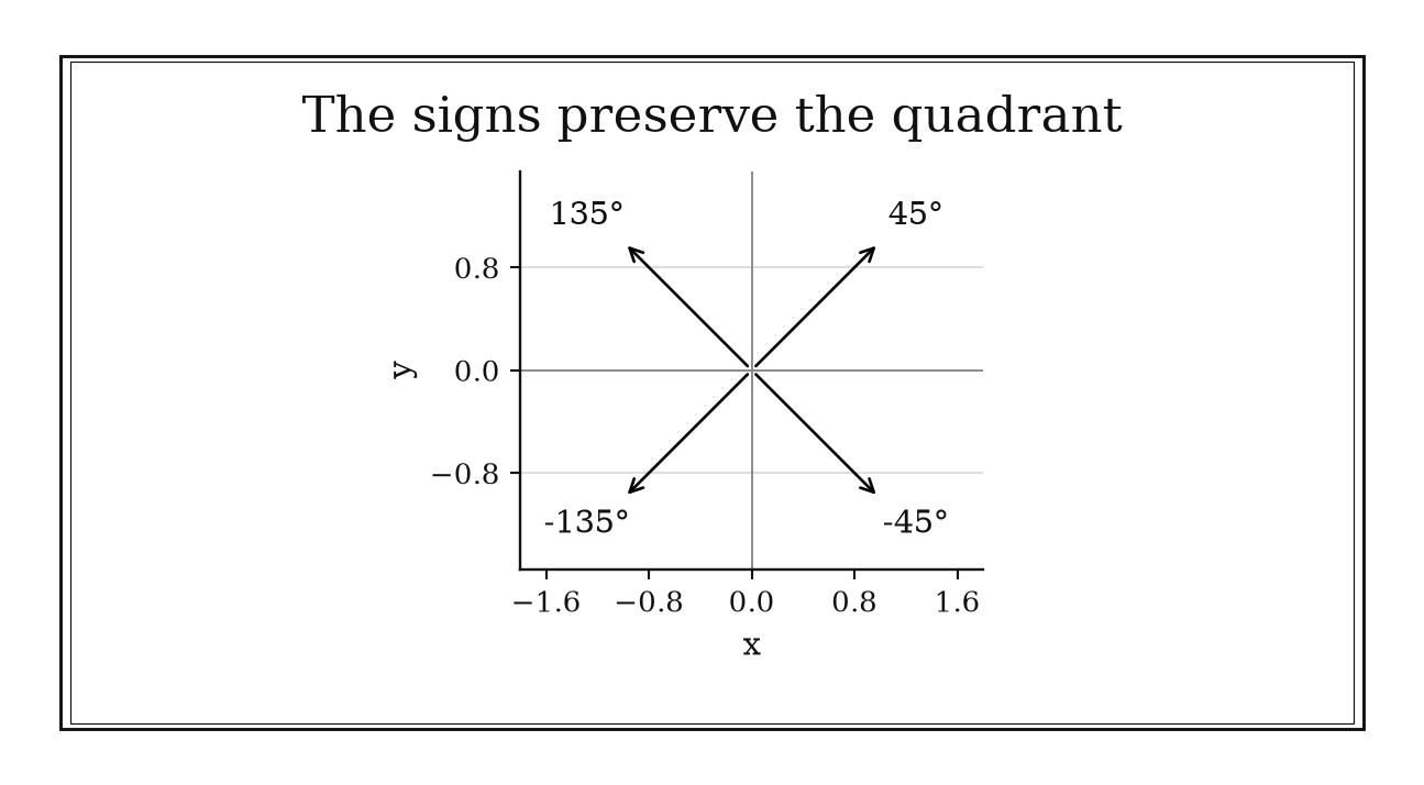
Figure 3.2. atan2 keeps the signs of both components. Opposite vectors have the same quotient y/x but headings separated by 180 degrees. The zero vector has no geometric heading.
3.2.2: Combine a sine-cosine pair into one shifted sinusoid
History
A sine term and a cosine term at the same frequency look like two separate signals needing two unrelated numbers. One oscillation should not need two. Leonhard Euler dissolved that appearance in his 1748 Introductio in analysin infinitorum, which organized exponential functions, trigonometric functions, infinite series, and complex quantities inside one common analytic language, making sine and cosine look like two coordinates of a single rotation rather than unrelated waves.
Euler’s Introductio establishes the analytic and complex connections behind this identity, though not the amplitude-phase shortcut itself: turning a sine-cosine pair into one shifted sinusoid for signal work is a modern packaging of his structure.
The equation
For real and ,
where
If , then and the phase is arbitrary.
How to read it
Expanding the shifted cosine gives . Matching coefficients requires and , and the Pythagorean identity gives . The pair is read as a point on a map: is the straight-line distance from the origin to that point, and is the bearing to it.
The identity preserves the complete oscillation; it just trades two component numbers for one amplitude and one phase, the way a distance-and-bearing pair replaces an east-north coordinate pair without losing information. It does not compress two different frequencies into one term: once appears, no single and reproduce both terms at once.
How to use it
An audio engineer mixes two same-frequency tones, one channel reading and the other , and needs the combined peak level before setting a limiter threshold. The amplitude is
with phase
so . The combined signal peaks at , not at or either channel’s own value, so the engineer sets the limiter just above instead of over-provisioning headroom for a peak that never occurs.
A quick coefficient check protects the phase’s quadrant:
both positive, confirming quadrant I. A plain applied to coefficients of mixed sign could land in the wrong quadrant, shifting the predicted peak by a half cycle, a phase error that shows up as audible smearing once mixed with a third track. The rule only merges terms sharing one frequency; a harmonic overtone at twice the frequency needs its own accounting. This is an Independent rule: the transformed sinusoid directly exposes amplitude, phase, and range across many periodic applications.
3.2.3: Reduce large angles before evaluating trigonometric functions
History
Ptolemy’s star tables could hold only so many angles; the sky refused to stay within them. His Almagest, compiled around the year 150 in Alexandria, answered that mismatch with a table of chords paired with symmetries and angle relations, letting a limited set of rows answer far more questions than they listed outright.
Ptolemy’s table and identities are directly documented. This rule belongs to the modern computational workflow that reduces a sine, cosine, or tangent argument to a convenient interval before evaluating it, in notation his tables never used.
The equation
For any integer ,
while
Sine and cosine repeat after a full turn; tangent repeats after a half-turn.
How to read it
Adding a full turn, , returns to the same point on the unit circle, the way walking around a circular track brings you back to your starting marker unchanged. After adding only a half turn, , both Cartesian coordinates flip sign, so their ratio stays the same; that is why tangent repeats twice as often as sine or cosine. Reduction preserves the function’s value exactly while revealing a smaller reference angle or an exact special value hiding inside a large input.
The function in play determines the most convenient period to subtract. Reducing tangent modulo remains valid but may leave a less convenient angle; reducing sine or cosine by an odd multiple of reverses its sign. The rule does not choose the right modulus for you.
How to use it
An observatory’s telescope-control software accumulates a mount rotation of radians after repeated slews and needs a quick check on the current pointing angle. Subtracting two full turns, , gives
Reduced angle falls in quadrant IV, where cosine is positive, matching the result and confirming the mount points roughly short of due east, not into the western sky. The operator proceeds with the exposure instead of halting to re-home the mount.
The shortcut misleads if the accumulated angle comes from a long run of floating-point slews rather than an exact value: at very large angles, the stored number may no longer carry enough low-order precision for the subtraction to land on the true remainder, so a control system that reduces modulo without re-homing against a fixed reference can drift into a confidently wrong pointing angle. This is a Workflow rule: range reduction prepares a simpler and often safer evaluation, but another identity, table, or numerical routine usually completes it.
3.3: Solve Triangles Without Losing Cases or Precision
A triangle may be determined, impossible, or ambiguous depending on which measurements are known. Even when the geometry is unique, a poorly chosen algebraic form can lose precision. These four rules preserve the included angle, the second inverse-sine branch, the natural angle unit, and a small positive difference.
3.3.1: View the law of cosines as corrected Pythagoras
History
A star’s triangle is rarely right-angled, and plain Pythagoras fails it outright. Solving that at Ulugh Beg’s Samarkand observatory in the 1420s needed a correction term; al-Kashi’s Key of Arithmetic and Treatise on the Chord and Sine record procedures for a triangle’s unknown side or angle, among them a form of what we now call the law of cosines.
The documented material is his triangle-solving procedure; naming it corrected Pythagoras is a later reading that separates the sum of squares from a correction sized by the angle’s departure from square, needed whenever a star’s triangle was not right-angled.
The equation
If side lies opposite the included angle between sides and , then
At , , and the equation becomes the Pythagorean theorem.
How to read it
The term is the correction on the familiar sum of squares. For an acute included angle, cosine is positive, so : the third side falls short of the right-triangle diagonal, the way a hinge closed tighter than square pulls its far corner inward. For an obtuse angle, cosine is negative, so , and the far corner swings outward instead.
The same relation handles two-sides-and-included-angle data directly and rearranges to recover an angle from three known sides. It only works when the angle used is the one actually included between the named sides; a different angle from the same triangle is a labeling error, not a rounding one.
How to use it
A land surveyor has staked two property-line segments of and chains meeting at a fenced corner where the included angle measures , and needs the third boundary’s length before drafting the plat.
so chains. Because the included angle is acute, should fall short of the right-triangle diagonal chains, and it does, confirming the field reading before it goes on the plat.
The formula misleads if the crew recorded the angle at the wrong corner: the reading must sit between the -chain and -chain segments, or the computed side belongs to a triangle that does not exist on the ground. When the included angle is small and the two sides are close in length, as with a nearly straight fence line, the formula subtracts two large nearly equal numbers to find a small result; the equivalent form avoids that cancellation, anticipating Rule 3.3.4. This is an Independent rule: given valid SAS or SSS data, it directly returns the missing side or angle across surveying, geometry, mechanics, and navigation.
3.3.2: Check both branches in the sine-law ambiguous case
History
Stopping at a calculator’s first answer can throw away half of the valid geometry. Precise triangle-solving carried real stakes for Jamshid al-Kashi’s astronomical work under Ulugh Beg in fifteenth-century Samarkand, where his writings on the chord and sine supported the triangle procedures positional astronomy demanded.
Those sources support al-Kashi’s careful triangle computation; the material does not show him stating today’s warning to check a second arcsine branch. That warning is a method-selection lesson added here, following from a plain fact: a numerical inverse sine reports only one principal angle even though the same positive sine value belongs to two different angles inside a triangle’s possible range.
The equation
The law of sines says
If it produces with , test
Retain only branches for which all triangle angles remain positive and sum to .
How to read it
Sine has the same positive value in quadrants I and II, since , the way two hinge angles on either side of a right angle can swing a door to the same height. An inverse-sine function usually returns only the smaller, acute value. Under SSA data, two sides and a nonincluded angle, the supplementary angle may complete a second valid triangle, or push the remaining angle to zero or below, ruling that branch out. The same measurements can therefore describe zero, one, or two genuinely different triangles, and the rule does not tell you which case you are in until you test both branches.
How to use it
A city planner knows an km City-Hall-to-water-tower line, a angle it makes with the sightline from City Hall to a proposed cell-tower site, and the site’s km distance from the water tower, and needs the City-Hall-to-site distance before signing a lease. The law of sines gives
The two candidates are
leaving and , both positive, so both configurations are valid. Since ,
Stopping at the first arcsine would have handed the planner only the km City-Hall-to-site distance, discarding a second siting km closer, the gap the lease decision hinges on.
Before filing either figure, the planner checks that the largest of all three solved sides faces the largest angle; rounded field measurements can also push the sine ratio just outside , a sign that the stated measurements are inconsistent and their uncertainty needs checking. This is a Workflow rule: it guards a larger triangle-solving procedure against silently losing or inventing a geometric solution.
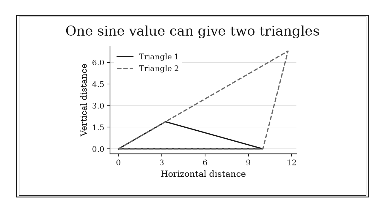
Figure 3.3. For A=30 degrees, a=7 and b=10, both positive solutions for the third side produce valid triangles. A single arcsine result would miss the second configuration.
3.3.3: Use radians whenever angles enter calculus or approximation
History
Feed a bare number into a calculus formula without asking its unit, and a derivative comes out wrong by a factor of over fifty, with no error message to flag it. Between 1869 and 1874, in Britain, the name radian emerged for the angle subtending an arc equal to its own radius: James Thomson used it in examinations by 1871, and Muir put it into print in 1874, a history later recorded in a Nature correspondence.
That episode documents the unit’s name, not why it matters: carries no extra factor only in radians, a fact independent of what the unit was called.
The equation
Convert degrees by
In radians,
and the small-angle relations begin and . If a numerical variable is measured in degrees instead, then
How to read it
Radian measure is the plain ratio of arc length to radius, , a number with no physical units of its own, the way a ruler marked in matching units on both axes makes a graph’s slope mean what it looks like. Degrees remain valid for reporting an angle to a person, but calculus must carry an explicit conversion factor whenever degrees are the numerical input.
The danger is not using degrees; it is silently inserting a degree number into a formula built for radians. The rule does not protect you from that mistake; it only tells you the factor is exactly once you look for it.
How to use it
A machinist commissioning a rotary table receives a spec sheet listing an angular speed of per second and needs the tangential speed of a workpiece at radius meters before setting a cutting tool’s feed rate. Converting first,
Tangential speed is , so
The machinist sets the feed to roughly m/s, not the raw that a unit-blind substitution would give.
That figure is the trap: plugging the unconverted straight into overstates the true speed by a factor of , with no warning, since the arithmetic runs without complaint either way. Labeling every angular variable with its unit, degrees on the spec sheet, radians in the formula, is what catches the substitution first. This is a Workflow rule: radian conversion prepares correct local and calculus operations across mechanics, waves, geometry, and numerical analysis.
3.3.4: Use a half-angle identity for one minus cosine
History
The identity is the artifact behind this rule: swap in the right-hand side, and a subtraction that silently destroys precision turns into a squared sine that cannot lose it. No dated computation or failure report records who first reached for that swap. Half-angle identities are classical algebra, but rewriting to defeat floating-point cancellation is a modern numerical-stability tactic, and the sources available turn up only later explanations of the identity, not a primary computation or error report where this rewrite was the corrective step. That leaves an evidence gap: closing it would need a code listing or error report showing someone reaching for this identity to fix a cancellation problem, dated with confidence.
Until such a record surfaces, the honest description is folk numerical practice, a stability trick spread through shared code long before anyone wrote down who reached for it first.
The equation
The half-angle identity gives
For small in radians, Rule 3.1.1 then gives
The next series correction is .
How to read it
The left side, , subtracts two numbers that sit close together whenever is small, the way subtracting two nearly identical bills to find a one-dollar difference leaves you unsure of the cents. In finite-precision arithmetic, that small residual may retain far fewer meaningful digits than either input carried. The right side, , represents the same value as a small sine’s square, making its nonnegativity and true scale explicit instead of leaving them to survive a subtraction. The identity is exact for every ; only the final replacement of sine by its own argument requires a small radian angle, and since that behavior is quadratic, the result cannot be replaced by a signed linear term. It does not fix a badly measured input; it only stops the arithmetic from destroying precision the input already had.
How to use it
A precision rifle-sports analyst measures a scope cant of radian and needs the vertical shortfall of a cm drop correction before recommending a re-mount. Direct subtraction would ask a calculator to subtract two numbers agreeing to about six decimal digits, risking a result with almost no reliable digits left. Using the exact identity instead,
That fraction of cm is only
vertically; the horizontal miss cm is similarly tiny, both far below what the scoring rings can register, so the analyst tells the shooter the cant is negligible. The same rewrite stabilizes the law-of-cosines form in Rule 3.3.1.
The identity does not rescue a badly calibrated gauge: if the sensor reports to only three reliable digits, no stable arithmetic recovers digits the measurement never had. This is a Workflow rule: it supplies an exact safer representation that supports a later evaluation, limit, or model calculation.
Chapter Synthesis: Preserve the Circle While Simplifying It
The rules in this chapter are not one triangle-solving algorithm. They are a set of controls on representation.
Near zero, ask whether the angle is in radians and whether the first omitted term is small enough. When direction or phase matters, keep both signed components until the quadrant has been selected. When the argument is large, remove full periods before doing detailed work. When triangle data produce an inverse function, remember that the calculator reports a branch, not necessarily every geometric solution. When a small answer is formed by subtracting nearly equal quantities, search for an exact identity that exposes the small scale directly.
Four checks organize the chapter:
- What angle unit makes the local geometry natural?
- Has any sign, quadrant, period, or inverse-function branch been discarded?
- Is the proposed simplification exact or approximate, and what is its first neglected term?
- Does this rule answer the question, or prepare a safer next calculation?
The first six rules often return an estimate, direction, amplitude, or side directly. The last four include independent triangle information and workflow guardrails. Keeping those roles distinct prevents a useful preprocessing step from being mistaken for a finished solution.
One-Page Trigonometry Toolkit
| Recognition cue | Rule to try | What it gives | Role |
|---|---|---|---|
| Small radian angle inside sine | Linear deflection with relative error scale | Independent | |
| Small loss from cosine’s maximum | Quadratic projection or phase loss | Independent | |
| Shallow slope or elevation | Angle-slope conversion with correction scale | Independent | |
| Direction from two signed components | Quadrant-aware direction | Independent | |
| Same-frequency sine and cosine | Convert to | Amplitude, phase, and range | Independent |
| Large periodic argument | Reduce modulo the correct period | Reference angle or safer input | Workflow |
| Two sides and their included angle | Correct Pythagoras with | Missing side or angle | Independent |
| SSA triangle data | Test both arcsine branches | Complete set of possible triangles | Workflow guardrail |
| Angle enters calculus or a local model | Convert degrees to radians | Natural derivative and approximation scale | Workflow |
| Small | Use | Exact stable nonnegative form | Workflow |
Decision Path
- Is the angle small? Convert to radians. Use sine or tangent as only after checking the cubic correction; use when cosine’s small departure from one matters.
- Are two signed components defining a direction or
phase? Preserve both with
atan2. If they multiply same-frequency cosine and sine terms, convert the coefficient pair to amplitude and phase. - Is the angle large or outside a familiar interval? Reduce it modulo the function’s period before using a reference angle or numerical routine.
- Is the triangle given by SAS or SSS? Start with the law of cosines. If it is given by SSA, use the law of sines and test both inverse-sine branches.
- Does the formula subtract nearly equal trigonometric values? Search for an exact identity such as before evaluating.
Transfer Problems
1. Build a small-angle error budget
A sensor tilts by . Estimate , , and using the rules in Section 3.1. Convert the angle once, write the first omitted term for each approximation, and decide which estimates plausibly support four decimal places.
2. Recover a signal’s amplitude and phase
Rewrite
as one shifted cosine. Use a quadrant-aware phase, state the range, and identify where the maximum first occurs in . Explain what would go wrong if the phase were computed only from .
3. Choose every valid triangle
A triangle has , , and . Determine whether the measurements produce zero, one, or two triangles. Before calculating the remaining side, list every inverse-sine branch and test it against the angle sum. Then state which rule you would use if the data instead supplied , , and the included angle .
Where These Ideas Reappear
- Calculus: the three small-angle formulas become Taylor models with systematic remainder control.
- Complex analysis and signal processing: amplitude-phase conversion becomes complex magnitude and argument, phasors, and Fourier representation.
- Linear algebra and geometry:
atan2is the two-dimensional version of preserving direction before normalizing coordinates. - Numerical methods: range reduction and the half-angle identity exemplify stable reformulation before floating-point evaluation.
- Differential equations and mechanics: small-angle sine produces linear oscillators, while its neglected terms explain amplitude-dependent corrections.
- Navigation, surveying, and astronomy: the laws of sines and cosines turn angular observations into distances, provided quadrants and branches remain intact.
Historical Notes and Sources
Sources for the historical accounts in this chapter follow. The half-angle entry supports the mathematics without claiming an unverified originating event.
- Huygens and pendulum isochronism: Smithsonian Libraries digitization of Huygens’s 1673 Horologium Oscillatorium; NIST reconstruction of Huygens’s pendulum timepiece.
- Al-Kashi and Samarkand trigonometry: MacTutor biography of Jamshid al-Kashi; MacTutor history of trigonometric functions.
- IBM’s two-argument arctangent: IBM
System/360 FORTRAN IV library manual documenting
DATAN2. - Euler’s analytic trigonometry: Euler Archive record for the 1748 Introductio in analysin infinitorum; MAA Mathematical Treasures discussion.
- Ptolemy’s chord table and identities: MacTutor history of trigonometric functions.
- The naming of the radian: Nature correspondence on the origin of the word; MacTutor mathematical-word history for “radian”.
- Evidence-gap mathematics: OpenStax, Precalculus 2e, Chapter 5 key concepts and Chapter 7 key concepts. These establish the identities and triangle relations but do not document a historical event in which the half-angle rewrite was adopted specifically to prevent numerical cancellation.