Chapter 4 , Calculus: Turn Local Change into Global Control
Without evaluating a square root, estimate . The nearby value is known, and the slope of at is . An input increase of should therefore produce an output increase of about , giving . The actual value is about .
That tiny calculation captures calculus at its most reusable. A derivative turns nearby change into a prediction. A derivative bound turns local slope information into a guarantee across an interval. Convexity traps a function between simple lines. An integral converts local contributions into accumulated effect, while comparison and symmetry can control that accumulation without an antiderivative.
The seventeen rules in this chapter fall into three families. The first builds local models and sensitivity estimates. The second reads global shape from derivative signs, convexity, and boundary growth. The third controls integrals, series, and method choice. Together they support one governing habit: use local information to make global decisions.
Calculus is not merely a catalogue of operations. Its deeper value is knowing what a slope, bound, comparison, or first omitted term licenses, and what it does not.
4.1: Build Useful Local Models
A curve viewed closely often behaves like its tangent. The four rules in this section turn that local resemblance into estimates, root corrections, percentage sensitivities, and hard change bounds.
4.1.1: Linearize near a point you already understand
History
Freeze a changing quantity at an old value, and an estimate quietly stops tracking reality the moment the input moves on. Between 1665 and 1671, working at Woolsthorpe and Cambridge, Isaac Newton developed methods of fluxions and infinite series connecting changing quantities, tangents, quadratures, and local approximation. Much of it circulated in manuscript before later publication, yet it became one foundation of differential calculus. Newton used tangent and series methods explicitly to read nearby behavior from a point already understood; the compact linearization formula below, and its error language, are later, more explicit expressions of that habit, not his own notation.
The equation
If is differentiable at , then for a small increment ,
The linear approximation is therefore
If a reliable second derivative is available, the leading correction is often .
How to read it
The known value is the answer at a point you already trust, and the slope converts a small step into a predicted output step, . The leftover term shrinks faster than itself as shrinks toward zero. What the formula does not say is how large a step still counts as close enough for the accuracy a given job needs; differentiability guarantees the trend, not a distance.
Pick the expansion point partly for convenience: a nearby perfect square, a familiar angle, or a tabulated value can make both and mental arithmetic.
A quick units check catches assembly mistakes: carries output units per input unit, so must carry the same units as . A mismatch means the local model was built wrong before any number was plugged in.
How to use it
A quality inspector on a machining line measures a shaft blank’s verified square cross-sectional area at square centimeters, against a nominal , and needs the equivalent side length before checking the shop’s tolerance chart. This is the chapter’s opening estimate at work: with , , ,
The chart allows a side length up to cm, so the inspector passes the blank without running an exact square root. The next correction,
predicts cm, confirming the tangent estimate runs slightly high.
Use linearization for mental arithmetic, calibration checks, and first-order uncertainty propagation, measured on the function’s own scale: a numerically tiny step can still cross a corner or region of rapid curvature. Had the tolerance been tighter than that quadratic correction, the quick estimate alone would not have been trustworthy. This is an Independent rule: once a trustworthy nearby point is chosen, it directly produces an estimate across many applications.
4.1.2: Interpret a Newton step as the tangent-line root
History
One tangent-line correction can land within thousandths of a true root, cutting many algebraic passes down to one. Newton produced that shortcut in De analysi, written in 1669 at Cambridge: an iterative method for improving an approximate root by substituting a correction term, keeping the part that controlled the answer, and dropping the rest as negligible. Joseph Raphson later recast the process in a form closer to the update taught today. Newton’s correction process is equivalent in substance to local linearization, though the derivative quotient and the geometric tangent-root picture are later standardizations, not his own algebra.
The equation
At a current estimate , linearize
Setting the right side to zero gives Newton’s update:
Near a simple root and under suitable smoothness, the error typically becomes proportional to the square of the previous error.
How to read it
The quotient carries the units of : it estimates how far the current guess sits, horizontally, from where the curve actually crosses zero. Subtracting it moves the guess to where the local tangent line crosses the axis instead. A steep slope gives a modest correction, while a nearly flat one can fling the next guess far from where it started.
What the step actually solves is the tangent’s equation, not the original curve’s equation: a step can look small and still be a poor guide to the real root once the tangent has drifted from the curve. Its speed comes from rebuilding that tangent after every step, never from touching the nonlinear equation directly.
How to use it
A venture analyst wants the annual growth factor that would double a portfolio company’s revenue over exactly two years, the positive root of . Starting from a guess , with and ,
A second step gives about , close enough to quote as a required growth rate of about per year. Before trusting it, the analyst checks the residual rather than just the size of the correction: a small correction can be misleading when the derivative is poorly scaled, while a small residual confirms the equation itself is nearly satisfied. A nearly flat slope on an early guess, or a tangent pointing outside a bracket already believed to contain the answer, is reason enough to reject a step rather than accept it blindly.
Newton’s method earns its use once a credible starting bracket exists. Poor starts, flat derivatives, or multiple solutions in a more complicated growth model can cause slow convergence or divergence, so in decision-critical work the analyst keeps a bracket and rejects any step that leaves it. This is a Workflow rule: the tangent-root interpretation selects and diagnoses one step inside a larger iterative solution.
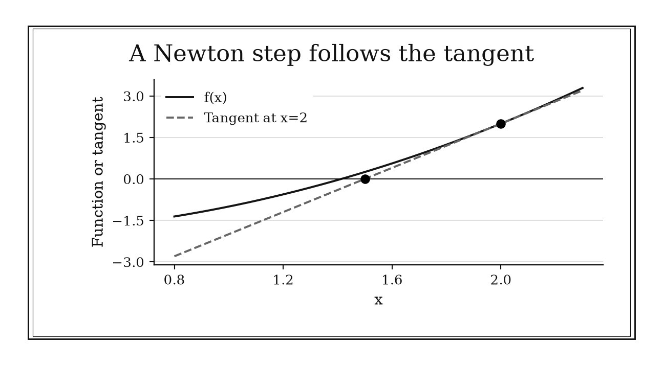
Figure 4.1. For f(x)=x²-2, the tangent at x=2 reaches zero at x=1.5. That improves the estimate but still differs from sqrt(2); later steps and a stopping check remain necessary.
4.1.3: Use relative differentials for power-law sensitivity
History
Notation is supposed to be neutral bookkeeping, a record of a calculation already understood elsewhere. Leibniz’s own symbols argued otherwise. His differential calculus appeared in 1684 in a Leipzig journal, with an account of integral calculus following in 1686, and his notation made the differential structure of products, composites, powers, and accumulated sums visible and directly manipulable. Leibniz supplied that differential language; turning a product of powers into a compact percentage-sensitivity checklist is a modern operational use of it, with the first-order assumptions stated explicitly. The payoff is practical: a design with several changing dimensions reduces to which single measurement matters most.
The equation
For positive reference values in
take logarithms and differentiate:
With more factors, add one exponent-weighted relative change for each factor.
How to read it
Each exponent acts like a percentage multiplier tuned to its own input. If , a small nudge in contributes roughly to ; a negative exponent flips that contribution’s direction. Because logarithms turn a product into a sum, contributions from several inputs simply add at this first-order level, one term per factor.
What this gives is signed sensitivity, not a worst-case bound: it flags which input’s error matters most, not the largest error several inputs could jointly produce. For finite fractional changes and , the exact scale factor is
where is the new value of , not a derivative, showing precisely which squared and cross terms the differential version leaves out.
The exponent-weighted coefficients are elasticities, percentage-change ratios rather than raw units: ranking them by size flags which input deserves the tightest measurement before any change is supplied.
How to use it
A concrete contractor is pouring a cylindrical silo column, and the formwork crew reports the radius will likely run over spec while the height runs short. Volume follows , so
The contractor reads this as the order being fine as specified, since the radius error carries twice the weight of the height error and the two nearly cancel. The exact scale factor,
confirms a decrease of only about , close enough to zero that no extra truck gets called.
Relative differentials answer exactly this kind of tolerance question, and flag which measurement, here the radius, deserves the tightest control on site. The formula assumes small fractional changes and a nonzero reference size; it does not say when “small” has stopped being small. If a form panel bows and the radius error grows to , the first-order cancellation can no longer be trusted, and the contractor should compute the exact ratio, since the very quadratic terms this rule discards can then become the whole story. This is an Independent rule: it directly estimates percentage response for power-law models across science, engineering, and finance.
4.1.4: Turn a derivative bound into a change bound
History
How much can a function possibly change, given only a ceiling on its slope? Newton’s tangent-and-series manuscripts from the 1660s already used local slopes to infer how a changing quantity behaved nearby, establishing the local idea long before anyone wrote today’s polished inequality. That inequality, which turns a single slope ceiling into a guarantee across an entire stretch, belongs to the later, rigorous account built around the mean value theorem. The payoff is a certificate that needs no formula at all: bound the slope everywhere on an interval, and no secant across it can exceed the same rate.
The equation
If is continuous on the closed interval between and , differentiable inside it, and
throughout that interval, then
How to read it
The mean value theorem guarantees some intermediate point between and where the secant slope equals the derivative there,
Because that unknown is still covered by the ceiling , bounding every slope on the interval bounds the total change. Where linearization predicts behavior near one point, this inequality is a certificate across the whole stretch between and , whenever its hypotheses hold.
A smaller valid tightens the result, but the bound never reveals the sign or exact size of , only a ceiling on it; the real value still needs evaluated directly.
The inequality also reads as a stability statement: two nearby inputs cannot produce outputs farther apart than times their separation, the same idea that becomes a Lipschitz bound in Chapter 5.
For example, has on , so
The interval matters as much as the starting point.
How to use it
A solar-monitoring technician models a panel’s relative output as proportional to , where is the sun’s elevation angle in radians, and needs to know how far a small angle-sensor error could shift the reading. Because for every angle,
so a sensor drift of radian cannot move the modeled output by more than on that same scale, with no trigonometric evaluation required.
Apply this over the whole angle range the uncertainty could reach rather than at the nominal reading alone: if a passing cloud makes the sensor’s output jump rather than vary smoothly, the continuity this argument relies on breaks. A loose but honest guarantee still beats an unsupported number that merely looks precise. This is an Independent rule: it directly converts a local rate ceiling into a transferable global change guarantee.
4.2: Read Shape from Derivatives and Convexity
Local slopes organize an entire graph when their signs or ordering are known. The three rules in this section use derivatives to locate rises and falls, convexity to build two-sided bounds, and boundary rates to estimate thin geometric layers.
4.2.1: Use the derivative sign before solving for extrema
History
Newton’s manuscript on fluxions, circulating privately between 1665 and 1671, already linked a rate of change to a curve’s tangents, its quadratures, and its behavior near a point. That body of work, published only later, helped found differential calculus. Reading a rate’s sign as a verdict on where a curve climbs, falls, or turns is the modern extension of that habit, formalized today through the mean value theorem into a systematic sign chart.
The equation
On an interval where the required hypotheses hold,
Partition the domain at points where , where does not exist, and at relevant endpoints.
How to read it
A single, unchanging derivative sign across an interval forces every secant slope there to share it, through the mean value theorem: positive throughout means the function only climbs, negative throughout means it only falls. An extremum shows up as a change of sign, positive to negative for a local maximum, negative to positive for a local minimum.
A zero derivative by itself is only a candidate, not a verdict: has derivative zero at the origin yet keeps climbing straight through it. Corners and cusps can also hide an extremum where no derivative exists, so those points need checking directly.
Repeated factors inside often predict the sign pattern without extra work: an odd-multiplicity factor usually flips sign as its root is crossed, an even-multiplicity factor usually does not, though a test point on each interval remains the final check.
How to use it
A logistics manager tracks a delivery route’s efficiency index as , where counts stops added to or cut from the route’s baseline, negative for cuts and positive for additions. Rather than solve the model directly, the manager reads
for its sign: positive below , negative between and , positive above , so the index rises, falls, then rises, peaking after cutting one stop at and bottoming out after adding one at .
The sign chart only ranks nearby options. Before locking in a schedule, the manager still checks the index at the shift’s true endpoints, the most stops the trucks can carry and the fewest the contract allows, since an unchecked endpoint can beat both local extremes. Points where the model itself breaks down, such as a stop needing an extra vehicle, belong in the partition too. This is an Independent rule: it directly determines qualitative shape and local extrema from reusable sign information.
4.2.2: Bracket a convex function between tangents and secants
History
A safety margin built on a bound facing the wrong direction is a false promise: a quantity assumed to stay below some ceiling can already have crossed it. Johan Jensen closed that kind of gap, working in Copenhagen in 1905 and 1906 on a systematic account of convex functions and the inequalities between mean values: a convex graph lies below every chord drawn between two of its points, while any supporting tangent line lies below the graph itself. Jensen connected convexity to inequalities between averages explicitly; today’s tangent-secant “bracket” operationalizes that structure to estimate a convex function without evaluating it exactly.
The equation
For differentiable convex , a tangent at gives
For with , the chord gives
For a concave function, the geometric inequalities reverse.
How to read it
Convexity means slopes never decrease as you move right along the graph. A tangent line uses just one local slope and can never rise above the curve; a chord connecting two known points averages the slopes between them and can never dip below the curve there. Together the two lines become a lower and an upper certificate, with no evaluation needed in between.
The tangent bound travels as far as convexity and differentiability hold; the chord bound only applies between its own two endpoints, since its weight must stay between zero and one. What neither line tells you is how tight the gap between them is: a curve that hugs close to straight leaves tangent and chord nearly touching, while a sharply bending curve can leave a wide space between them.
For a point between and , the chord weight is ; moving either the chord’s endpoints or the tangent point closer to tightens the corresponding bound, so several known points can build a tighter, piecewise bracket.
How to use it
An epidemiologist facing an outbreak whose case count grows like over weeks needs a fast bound on the growth factor at weeks, without waiting on the full exponential model during a briefing. The tangent at zero gives
so at , , and growth is at least -fold. The chord through and over the first week gives
so at , , and growth is at most about -fold. The true factor, about , sits inside that bracket, which the epidemiologist can quote before the exact model finishes running.
The bracket holds only because the case-growth model is convex; the epidemiologist checks that with where available, and would split the timeline into separate windows once curvature changed sign, for instance after interventions started bending the curve down, since one global picture would no longer bound the new regime. For a concave process, such as cases approaching a saturation ceiling, the roles reverse: tangents lie above and chords below. This is an Independent rule: convexity directly supplies portable lower and upper bounds without exact evaluation.
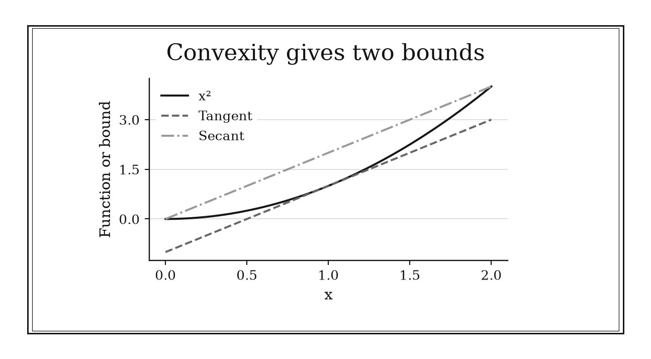
Figure 4.2. On [0,2], x² lies above its tangent at x=1 and below the secant joining the endpoints. The upper bound is restricted to the interval spanned by that secant.
4.2.3: Estimate a thin shell as boundary measure times thickness
History
An eyeballed estimate of a thin coating drifts further from the true volume the more curved the surface underneath. Around 250 BCE in Syracuse, Archimedes compared planar slices and solid sections through geometric balance arguments, preserved in The Method and related works, using infinitesimal-style decompositions heuristically before supplying geometric proofs acceptable by ancient standards. Archimedes did not write a modern shell differential; his documented slice-and-balance reasoning is the historical practice, and reading a thin boundary layer as boundary measure times thickness is the modern calculus translation of it. What that translation buys is a fast, first-order answer for any thin uniform layer, without rebuilding the whole solid from scratch.
The equation
For a circle of radius and small outward thickness ,
For a sphere,
More generally, a sufficiently thin uniform layer of thickness along surface area has leading volume
How to read it
The boundary measure is the rate at which interior measure grows when the boundary itself is nudged outward. Differentiating gives the circle’s circumference ; differentiating gives the sphere’s surface area . Multiplying that rate by a thickness gives the first-order layer.
What this shortcut leaves out is curvature: the omitted terms grow with how sharply the surface bends, so the estimate is only as good as the thickness is small compared with every relevant curvature radius.
The exact spherical expansion makes those omitted terms explicit:
Surface area times thickness is only the first term; curvature supplies the rest.
A units check confirms the setup before any number is plugged in: boundary area times length gives volume, and circumference times length gives planar area. A mismatch means the wrong boundary measure was used.
How to use it
A manufacturing engineer is specifying a radial allowance around a circular sheet-metal end cap, radius cm. The allowance extends the cap’s radius by cm. The quick estimate for the added planar area is
while the exact annulus area is
The missing is exactly the quadratic thickness correction, small enough here that the engineer budgets the additional sheet-metal area by the quick estimate and rounds up.
Boundary times thickness works for coatings, machining allowances, and other thin annuli or shells, but it assumes a small, roughly uniform layer and a well-behaved offset. On this same tank, a corner where the cap meets the cylindrical wall, or a spot where two coating passes overlap, would need a separate, exact calculation, since the local formula cannot see those topological changes or self-intersections. This is an Independent rule: it directly estimates thin-layer measure in many geometries without constructing a full volume integral.
4.3: Control Integrals, Series, and Method Choice
Accumulation problems rarely begin with antiderivatives. The ten rules in this section first ask what range, symmetry, endpoint motion, benchmark, or structural pattern can settle the question, or at least choose the correct procedure.
4.3.1: Check an integral average against the function’s range
History
A number that looks reasonable can still be wrong in a way no re-checked arithmetic will catch, unless it is tested against the one thing it cannot violate: the range of the function it came from. Augustin-Louis Cauchy built the tools for that kind of test. Working in Paris, his Cours d’analyse of 1821 and the calculus lessons that followed rebuilt differentiation, integration, and infinite series around limits, using inequalities and comparison to control convergence where earlier methods had often been used only formally. Cauchy treated limits, integrals, and series comparison explicitly; the compact “check the average against the range” wording here selects one of those mechanisms as a fast, first-pass audit.
The equation
For a continuous function on with , define
If on the interval, then
Continuity also guarantees some with .
How to read it
Multiply the inequality through by the interval’s positive length and integrate, and the total signed area gets trapped between and ; dividing back by returns everything to the function’s own scale. An average landing outside that range cannot be some unusual feature of the curve. It has to be an arithmetic, sign, unit, or normalization mistake. Passing the check is not the same as being correct: a wrong value can still land inside the range and slip through undetected.
The check is about average value, not the raw integral itself: on an interval whose length is not one, those two quantities live on different scales. If measures time and measures power, the integral carries units of energy; dividing by elapsed time restores power.
How to use it
A city water-utility analyst computes the average flow rate through a meter over a one-hour test as , where , in liters per second, ranges from to across the hour. With ,
which passes the range check at once, since sits between and . Over a longer two-hour test the same flow model gives an integral of and an average of
which still lies between the endpoints and , so the check passes here too, even though is the raw integral and not an average; mistaking one for the other would have gone undetected by this same check.
Run this test right after any hand or software integration, before quoting a flow rate as representative of the period. The same range bound holds for a normalized average with nonnegative weights and positive total weight. Signed weights do not guarantee it, and an unbounded monitoring window requires a separately defined averaging procedure. This is an Independent rule: it directly validates the scale of an accumulated result across many applications.
4.3.2: Exploit even and odd symmetry before integrating
History
Mechanical intuition and mathematical proof are not the same thing, and Archimedes kept the two separate. Writing in Syracuse in the third century BCE, in the treatise now surviving as The Method, he set matching cross-sections of a figure on an imagined scale, letting paired pieces on opposite sides of a center cancel or add, then followed that mechanical reasoning with a separate geometric proof built to satisfy ancient standards of rigor. Archimedes never wrote a signed integral or an even-odd identity; the symmetry rule used here is a later expression of that same instinct for weighing matched pieces against each other.
The equation
If and the integral exists, then
If , then
How to read it
Reflecting an even function across the vertical axis leaves it looking unchanged, so its two half-interval pieces reinforce each other when integrated. Rotating an odd function’s graph through the origin flips its sign, so equal contributions on opposite sides cancel in the signed sum.
That zero for an odd function is a statement about net accumulation, not about area: the positive and negative lobes on either side can each be large even while their signed total comes out to nothing.
Any function on a symmetric domain splits into an even part and an odd part,
and since the odd piece always integrates to zero, only the even piece’s half-interval integral, doubled, survives:
This extends the shortcut beyond functions that are purely even or purely odd. In numerical work, integrating only half a symmetric interval can nearly halve the computation, and pairing opposite sample points makes an odd component’s cancellation exact instead of leaving it to rounding.
How to use it
A sports biomechanics analyst models the net torque of a golfer’s downswing about its midpoint as over seconds, and needs the net rotational impulse over that symmetric window without integrating term by term. Since is odd and is even, making odd, the integrand is odd on a symmetric interval, so
without finding any antiderivative: torque in the first half of the swing exactly cancels torque in the second half.
Run this symmetry check before substitution, integration by parts, or numerical quadrature. A net of zero does not mean the torque itself was small: each half can carry a large, opposite torque that a coach still needs broken out, and a shifted window, say instead of one centered on the midpoint, would destroy the cancellation entirely. Taking the absolute value of an odd integrand also changes the conclusion, since is even where is odd, and the integral must actually exist for informal cancellation of two divergent halves to mean anything. This is an Independent rule: on a symmetric domain, parity can directly finish the integral across many settings.
4.3.3: Differentiate an accumulated integral at its moving endpoint
History
An accumulation with no closed formula for its running total can still be differentiated, once the endpoint doing the accumulating is treated as the real variable in play. Leibniz’s publications of 1684 and 1686 made composite change visible through notation, the same symbols that expressed differentiation rearranging to recognize accumulated change in a new variable. Leibniz established that calculus structure; scanning an integrand’s moving endpoint for the rate it is adding, rather than solving for the whole accumulated amount, is a modern reading built on it, with continuity and chain-rule hypotheses made explicit.
The equation
For continuous ,
With both limits moving,
How to read it
A small outward shift of the upper endpoint adds a thin slice of accumulation: its height is roughly the integrand’s value there, its width the endpoint’s own displacement, and the chain factor converts a step in into that displacement. A moving lower endpoint removes a slice instead, which is where the minus sign comes from.
What this derivative gives is the accumulation’s rate at a single instant, not the accumulated total itself; finding the running sum still requires the integral, closed form or not. In the simplest case, has : moving the endpoint one small step adds that much area. A continuous probability density gives its cumulative function the same property, .
How to use it
A simulation analyst studies the accumulated model response , where is a dimensionless control parameter and is a dimensionless integration coordinate. The integrand is a signed contribution density, so the analyst needs the response’s rate of change with respect to . Differentiating the accumulation directly gives
with the dummy variable disappearing only after evaluation at the endpoint; replacing it by too soon would obscure the chain. At , , so the accumulated response is locally increasing as the control parameter increases. As a two-endpoint check, if describes accumulation between two moving coordinates, , and each term records one endpoint’s contribution.
This rule works for net infusion rates, distance traveled, or any parameter-dependent accumulation, given the fundamental theorem’s regularity; a discontinuous absorption rate needs a more careful, almost-everywhere version. This is an Independent rule: moving-endpoint structure directly yields a derivative even when the accumulated function cannot be written elementarily.
4.3.4: Memorize the p-integral convergence threshold
History
This threshold traces to one document: Cauchy’s 1821 lecture program, which treated improper integrals and convergent series through explicit comparison and limiting arguments, giving a rigorous setting in which a vanishing term could finally be told apart from a finite accumulated tail. That framework is documented history; treating one power-law exponent as a universal pass or fail line is a present-day shorthand built on it.
The equation
At infinity,
Near zero, the direction reverses:
How to read it
For , the antiderivative contains , which settles to a finite value at infinity only when the exponent is negative, that is, when . At the boundary itself, the antiderivative is , whose unbounded growth creates the harmonic threshold.
An integrand shrinking to zero is not sufficient for its tail to converge: decays forever and still accumulates infinite area.
For , the leftover area beyond a cutoff is explicit,
which explains why convergence near can be painfully slow: the denominator is small and decays weakly. The threshold classifies convergence, while this explicit formula also sizes a pure power-law tail. Logarithmic factors require a separate comparison.
How to use it
An environmental engineer is tracking a contaminant’s concentration downstream of a spill, which decays like per unit distance past the outfall, and needs to know whether total exposure integrated out to infinity is even finite before running a full transport model. Since
the tail converges, though to a large finite value, while a nearby model with decay,
diverges outright: the tiny exponent difference crosses a real qualitative line, and both concentrations trending toward zero is not enough to tell the two cases apart.
The engineer first identifies which end of the domain is improper. Every fixed power is integrable on a finite stretch away from zero; the threshold only bites because one endpoint is singular or infinite, here the infinite downstream limit. A logarithmic correction in the real decay curve could also decide a borderline case where the exponent lands exactly at , so an exponent that close needs a sharper benchmark before the engineer signs off on bounded total exposure. This is an Independent rule: it directly classifies the model power integral and anchors convergence decisions throughout analysis.
4.3.5: Compare positive integrands with a known benchmark
History
A tail declared finite without a real certificate can leave a budget or a warranty resting on nothing. Cauchy grounded calculus in the limit concept, and his rigorous treatment of series and integrals let a positive, ever-shrinking quantity be checked against a known benchmark instead of summed or integrated outright. That comparison-under-limits program is the historical mathematics; the concise direction-check used here is a modern first-pass formulation of it.
The equation
For eventually nonnegative functions on a tail,
Conversely,
How to read it
For nonnegative functions, a taller graph accumulates more area: a function that never exceeds a convergent benchmark cannot itself blow up, and a function that never falls below a divergent one cannot itself stay finite. Only the direction that supports the conclusion is useful; running the comparison backward proves nothing.
Only the tail has to obey the inequality: a bounded initial stretch contributes a finite amount regardless and can be set aside. What the comparison never delivers is the integral’s own value, only whether it stays finite, and it works only as well as the benchmark in hand.
How to use it
A logistics network planner is estimating whether the total expected cost of increasingly rare, increasingly long shipment delays stays bounded, modeling the cost density of a delay of length days as . For ,
and since the benchmark converges, so does the planner’s tail cost, meaning a fixed reserve can in principle cover it. A rival model with cost density instead gives, for ,
a constant multiple of the divergent benchmark, so that tail cost has no finite bound at all, no matter how large a reserve is set aside.
When the comparison isn’t obvious by inspection, the planner can check the ratio of the candidate density to a benchmark as grows large: if it settles on some positive, finite constant, the two tails share the same convergence behavior, though that ratio is only a discovery tool, and the actual inequality still has to be shown to certify the answer. This works only while the cost density stays nonnegative on the tail; a density that can go negative would need an absolute-value or alternating-series treatment instead. This is an Independent rule: it directly transfers a known convergence verdict to broad families of positive integrands.
4.3.6: Bracket a decreasing series tail with integrals
History
Sum a slowly converging series by hand past a few hundred terms, and patience runs out long before the tail does. Cauchy’s rigorous, limit-based treatment of calculus and series turned that stall into an auditable claim, using inequalities and comparison to control convergence instead of demanding every term be summed by hand. That comparison discipline is documented history; the bracket below, pairing positive decreasing terms with neighboring areas, is the modern form of that discipline.
The equation
If is positive and decreasing and , then the tail after satisfies
The upper integral is a guaranteed truncation-error bound.
How to read it
Picture decreasing rectangles of width one stacked along the curve. A right-endpoint rectangle sits below the curve over the interval just before it, while the matching left-endpoint rectangle sits above the curve over the interval just after. Summing those comparisons traps every unseen rectangle between two neighboring improper integrals.
This bracket sizes an actual remainder, beyond confirming convergence, yet never evaluates the sum itself; if monotonicity lapses even briefly, the picture stops trapping anything. For a -series with , the general bracket becomes
which turns a target error tolerance directly into a term budget.
How to use it
A financial analyst values the tail of a structured settlement whose remaining payments shrink like for payment number , and needs a bound on the value left after the first payments without summing hundreds of terms by hand. Since
the remaining value is about in the payment’s own units, with the midpoint near , a bound obtained without summing the full schedule. If a client instead needs the value within , the upper bound alone shows that payments already suffice.
The bracket applies only once payments are positive and genuinely decreasing; an irregular first few, negotiated separately, can be pulled out and handled on their own. A stream that oscillates or occasionally increases calls for an alternating-series or absolute-convergence tool, and indexing matters: the first payment left out is , which sets both integral limits. This is a Workflow rule: it controls truncation inside a larger series computation and tells you when to stop.
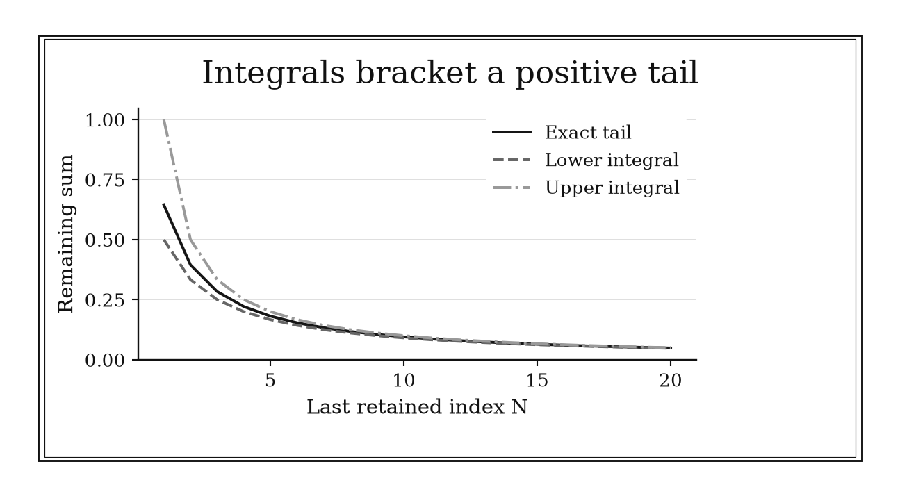
Figure 4.3. For the tail sum of 1/k² after k=N, integrating from N+1 gives the lower bound and from N the upper bound. The exact tail here is pi²/6 minus the finite partial sum.
4.3.7: Look for an inner function and its derivative
History
A composite integral that looks intractable can collapse to one line once its inner expression and that expression’s derivative are both spotted inside it. Leibniz’s published calculus of the mid-1680s let a compound expression be read and rearranged symbol by symbol, rather than treated as a single opaque block. That documented notation is the historical structure; the habit of searching an integral for the chain rule run backward came later, as a workflow reading of it.
The equation
If , then
With the substitution
the composite integral becomes .
How to read it
Substitution runs the chain rule backward: the inner function becomes the new coordinate, and converts a small step in into a small step in . A constant mismatch is harmless once corrected exactly; a variable mismatch is not.
Spotting the pattern must come before expanding anything: multiplying out a composite power or product can destroy the structure that would have collapsed the integral. What the rule does not do is say which inner function to try when more than one looks plausible; only trial and a differentiation check settle that.
Common signatures include , suggesting ; , suggesting ; and , suggesting a power of .
How to use it
A mechanical engineer computing the work done by a variable restoring force during a compression stroke needs , where is piston displacement in centimeters. Spotting and its derivative together, the engineer sets , so
Differentiating the answer confirms both the outer derivative and inner factor return, catching a dropped constant before it reaches a design report.
For a full stroke from to , transforming a related model’s limits via turns into , with no need to substitute back to . The scan works for powers, exponentials, logarithms, and rational expressions with a repeated inner form, but a derivative only resembling the needed factor, not matching it up to an exact constant, is not a match. For definite integrals, transform both limits into or back-substitute fully, never mixing an -limit with a -integrand. This is a Workflow rule: it chooses a representation and simplifies one stage of a broader integration problem.
4.3.8: Choose integration by parts to move complexity
History
Is a derivative something you assign, or something already latent in a product, waiting to be transferred? Leibniz’s published calculus treated products, sums, and composites as one shared symbolic system, and rearranging his product rule supplied the structural basis for shifting a derivative from one factor onto another inside an integral. Modern selection mnemonics and the phrase “move complexity” are later workflow guidance, not quotations from Leibniz.
The equation
From ,
A common selection order for is logarithmic, inverse trigonometric, algebraic, trigonometric, exponential, often remembered as LIATE, but simplification is the real criterion.
How to read it
Integration by parts moves the derivative onto whichever factor you call , chosen because its derivative gets simpler, while the factor assigned to needs a manageable antiderivative of its own. The mnemonic ranks common cases; it does not prove any particular choice optimal.
Sometimes two applications return the original integral. Let . Parts gives , and a second application turns the new integral into , so
and . Recurrence can be exactly the intended simplification, and repeated parts against a polynomial factor is especially predictable: each application lowers its degree until it disappears.
How to use it
Redevelopment pressure along a corridor grows like for distance in kilometers from the waterfront toward downtown, and a city planner needs to total that pressure over a stretch. Taking and gives and , so
Differentiating confirms ; the reverse assignment would integrate while differentiating , producing a higher-degree polynomial and no simplification.
Over the corridor’s first kilometer,
unit of pressure, above the review threshold, so the planner flags that block for review. Parts suits a polynomial paired with an exponential, logarithm, inverse function, or repeated trigonometric-exponential term; a poor choice of can reproduce or worsen the integral, which the planner then collects algebraically rather than abandoning it. This is a Workflow rule: it reallocates complexity within an integration procedure rather than independently answering every integral.
4.3.9: Use L’Hôpital only after confirming an indeterminate form
History
A ratio that vanishes on both top and bottom looks unsolvable until each part is differentiated separately, a shortcut whose credited author did not fully derive it himself. In Paris in 1696, the Marquis de l’Hôpital published Analyse des infiniment petits, the first textbook on differential calculus, including the limit rule bearing his name, based on results Johann Bernoulli supplied under their documented arrangement. The book presented the rule for certain vanishing ratios; the modern guardrail, verifying a genuine or before differentiating, is the precise operational lesson drawn from it.
The equation
Under L’Hôpital’s rule hypotheses, if a quotient has the indeterminate form or and the derivative quotient has a limit, then
The statement also has appropriate one-sided and infinite-limit forms.
How to read it
What the theorem transfers is a single limit under specific conditions, not a claim that a quotient and its derivative quotient are equal as functions; the link runs through a mean-value relationship between changes in numerator and denominator. Direct substitution must show indeterminacy first; an already-determined ratio should simply be evaluated as is.
Forms such as , , and are not quotients of the required type until rewritten as one. For example, has form ; rewritten as , an quotient, differentiating gives . The algebraic rewrite is part of the method, not a cosmetic prelude.
For powers such as , take a logarithm, convert the resulting product into a quotient if needed, evaluate, and exponentiate back, provided the domain permits the logarithm.
How to use it
A calculus tutor watches a student reach for L’Hopital’s rule on every limit in a problem set, including , already the determined form by direct substitution; differentiating anyway gives , the wrong answer, because the rule never applied there. On the actual indeterminate case in the same set,
substitution gives , and differentiating numerator and denominator correctly yields .
The tutor’s fix is a habit, not a formula: check substitution first, and reach for the rule only once a limit is genuinely indeterminate, since repeated use needs the hypotheses re-verified at each stage, and domain restrictions or zeros of the denominator’s derivative near the limit can still derail it. This is a Workflow rule, specifically a guardrail that selects a legitimate limit method and blocks a seductive invalid manipulation.
4.3.10: Use the first omitted Taylor term as an error scale
History
A single book title, Methodus incrementorum directa et inversa, is the documented artifact behind this expansion: Brook Taylor published it in London in 1715. Later analysts, especially Joseph-Louis Lagrange in Paris, developed systematic remainder forms separating a finite approximation from what had been left out. Taylor supplied the expansion; Lagrange’s era supplied the controlled remainder language. Treating the next term as an error scale is a modern rule still requiring regularity checks.
The equation
Taylor’s theorem writes
If between and , the Lagrange bound gives
How to read it
The first omitted term carries the next power of the small increment, making it the natural error scale when derivatives and coefficients behave regularly. That scale is not automatically a bound: a rigorous certificate still needs a derivative bound or, for a suitable alternating decreasing series, the alternating-series remainder theorem.
The rule also helps choose the expansion order: keep terms until the next credible contribution falls below the required tolerance. Choosing so that
separates two decisions, where to center the expansion, which sets and , and how many terms to keep.
For an alternating series with decreasing terms, the first omitted term is itself a rigorous bound and predicts the error’s sign too.
How to use it
A financial analyst approximates the growth factor for a continuously compounded return, , using terms through the quadratic:
The first omitted term,
predicts the error’s scale; the actual error is about , close but slightly larger than the term itself. A rigorous Lagrange bound, using on , gives an error below about , the figure the analyst would actually cite in a filing.
Use the first omitted term for order selection, quick error budgeting, and interpreting local approximations from Chapter 1, but verify the expansion point is not near a singularity and that the needed derivatives stay controlled. If successive terms are not shrinking, the next term may be a poor guide rather than a reliable one. This is a Workflow rule: it determines when a finite approximation is adequate inside a larger calculation.
Chapter Synthesis: From Local Information to Reliable Decisions
Calculus becomes portable when its operations are read as statements of control.
A derivative can make a prediction, produce a root correction, convert percentage inputs into percentage outputs, or impose a hard limit on total change. Its sign organizes rises and falls; the ordering of slopes creates convexity brackets; and the derivative of area or volume turns a boundary into the leading measure of a thin layer.
Integrals and series are controlled by equally structural questions. An average must remain inside the function’s range. Symmetry can reinforce or cancel contributions. A moving endpoint turns accumulated area back into a local rate. Power thresholds and positive comparison decide convergence without exact antiderivatives, while adjacent integrals quantify a series tail.
Finally, method rules protect formal manipulation. Substitution reverses the chain rule, integration by parts rearranges the product rule, L’Hôpital requires a verified indeterminate quotient, and Taylor truncation requires evidence about the omitted remainder.
The deeper habit is to separate four questions:
- Is the result an estimate, a bound, a classification, or a method choice?
- What interval or neighborhood must the hypothesis cover?
- What is the first neglected effect, and is it below the decision tolerance?
- Does local information genuinely control the larger object?
Those questions turn symbolic technique into mathematical judgment.
One-Page Calculus Toolkit
| Recognition cue | Rule to try | What it gives | Role |
|---|---|---|---|
| Nearby easy input value | Use the tangent line | Local numerical estimate | Independent |
| Approximate nonlinear root | Take the tangent-line root | Rapid correction step | Workflow |
| Product of powers with small percentage changes | Add exponent-weighted relative changes | Sensitivity estimate | Independent |
| Derivative bounded on a whole interval | Multiply slope bound by input distance | Hard change bound | Independent |
| Need rises, falls, or extrema | Make a derivative sign chart | Qualitative shape and candidates | Independent |
| Convex or concave function | Use tangents and chords | Two-sided function bounds | Independent |
| Thin uniform geometric layer | Multiply boundary measure by thickness | Leading area or volume change | Independent |
| Integral average | Compare with integrand range | Scale audit | Independent |
| Symmetric interval | Test even or odd parity | Doubling or cancellation | Independent |
| Integral with moving endpoint | Evaluate at each endpoint and multiply by its derivative; subtract the lower contribution | Accumulation derivative | Independent |
| Power-law improper integral | Compare exponent with one | Convergence threshold | Independent |
| Positive tail resembling a benchmark | Compare above or below in the useful direction | Convergence transfer | Independent |
| Positive decreasing series tail | Use neighboring improper integrals | Remainder bracket | Workflow |
| Composite integrand plus inner derivative | Substitute the inner expression | Chain-rule reversal | Workflow |
| Product with a simplifying derivative | Integrate by parts | Complexity transfer | Workflow |
| Quotient limit giving or | Check L’Hôpital’s hypotheses | Valid derivative-quotient route | Workflow guardrail |
| Truncated Taylor expansion | Inspect and bound the next contribution | Error scale or certificate | Workflow |
Decision Path
- Is the input near a value you understand? Linearize. If you are solving , interpret that linear model’s root as a Newton step.
- Is the question about sensitivity or guaranteed change? Use relative differentials for small percentage response; use a derivative supremum when a hard interval-wide bound is required.
- Is the question about graph shape? Partition at critical, nondifferentiable, and endpoint values. Use derivative signs for monotonicity and convexity for tangent–secant bounds.
- Is a thin layer being added? Multiply boundary measure by thickness, then compare the curvature correction with the tolerance.
- Before integrating, can structure finish the problem? Check range, parity, and moving endpoints before seeking an antiderivative.
- Is the issue improper accumulation? Identify the troublesome endpoint, recall the threshold, compare positive integrands in the correct direction, and use adjacent integrals when a decreasing series remainder is needed.
- Do you need an integration method? Search first for an inner function with its derivative, then consider whether parts transfers complexity profitably.
- Do you need a limit or approximation? Verify an indeterminate quotient before L’Hôpital, and verify a remainder condition before treating the next Taylor term as a bound.
Transfer Problems
1. Predict, then certify
Estimate with a linear model. Then use a Taylor remainder bound to certify the error and decide whether the approximation is trustworthy to three decimal places.
2. Read a graph without plotting it
For on , build a derivative sign chart, locate local and absolute extrema, and identify intervals where a tangent–secant convexity bracket can be used without crossing an inflection point.
3. Choose structure before procedure
For each object, name the first calculus rule you would use and justify its hypotheses:
For the first, compare symmetry with substitution; for the other two, give a convergence argument or numerical tail bracket without seeking unnecessary exact forms.
Where These Ideas Reappear
- Analysis: derivative bounds become Lipschitz control, and integral or series comparisons become formal convergence machinery.
- Asymptotics: linearization and Taylor remainders become systematic expansions ordered by a small parameter.
- Geometry: convexity, tangent lines, and thin shells recover the scale and curvature estimates of Chapter 2.
- Probability and statistics: moving-endpoint integrals define densities and distribution functions, while Taylor models drive the delta method.
- Optimization: derivative signs, convex bounds, and Newton corrections become algorithms with line searches and stopping rules.
- Numerical methods: remainder bounds, bracketing, and method selection become explicit error and stability controls.
- Differential equations: local slopes are integrated into trajectories, and derivative bounds control how errors grow in time.
Historical Notes and Sources
Sources for the historical accounts in this chapter follow. Every calculus rule has a verified historical connection; the concise decision language and modern hypotheses remain later interpretations.
- Newton on fluxions, series, and local change: The Newton Project digital manuscripts and MacTutor, “The Rise of Calculus”.
- Newton’s root iteration: MacTutor biography of Isaac Newton and The Newton Project editorial context.
- Leibniz’s differential and integral calculus: MacTutor, “The Rise of Calculus” and MAA Convergence on Leibniz’s calculus papers.
- Jensen and convex functions: Jensen’s original paper, Sur les fonctions convexes and MacTutor biography of Johan Jensen.
- Archimedes on slices, balance, and symmetry: Archimedes Palimpsest project on The Method and Harvard Archimedes translations and studies.
- Cauchy on limits, integrals, and series comparison: Bibliothèque nationale de France record for Cours d’analyse and MacTutor biography of Augustin-Louis Cauchy.
- L’Hôpital and Johann Bernoulli: MacTutor biography of Guillaume de l’Hôpital and MacTutor biography of Johann Bernoulli.
- Taylor expansions and Lagrange remainders: MacTutor biography of Brook Taylor and MacTutor biography of Joseph-Louis Lagrange.
- Modern calculus statements and worked forms: OpenStax on linear approximations and differentials and OpenStax on improper integrals. These support the modern mathematics, not the exact historical phrasing of the rules.