Chapter 5: Analysis: Know When Limits and Proofs Are Safe
A sequence of continuous curves can converge at every point and still leave a discontinuous curve behind. A family of ever-narrower continuous spikes can approach zero at each fixed point while keeping the same total area. A sequence can settle down so completely that its terms become arbitrarily close to one another, yet fail to converge because the space containing it has a hole.
These are not technical tricks. They expose the question at the center of analysis: what control survives a limiting process? A plausible calculation can fail because its bound depends on the point, its convergence occurs in the wrong space, or its quantifiers were silently rearranged. The cure is not more symbolism. It is to state exactly what is controlled, where it is controlled, and whether the control is strong enough for the next step.
The twelve rules in this chapter form three families. The first turns continuity and contraction into numerical error bounds. The second routes convergence questions toward tests that match the available evidence. The third treats proofs as designed objects: identities are extended from dense sets, claims are negated one quantifier at a time, induction hypotheses are strengthened, compactness prevents escape, and delta is chosen from the error target rather than guessed.
The governing habit is simple to say and demanding to practice: before passing to a limit or completing a proof, identify the uniform bound, completeness property, or logical dependency that makes the passage safe.
5.1: Quantify Stability Before Trusting Approximation
Continuity says nearby inputs have nearby outputs. For practical work, that promise becomes much more useful when “nearby” is assigned a number. The three rules in this section turn regularity into an error budget, iteration into a stopping certificate, and pointwise convergence into a warning that stronger control may be needed.
5.1.1: Use a Lipschitz constant as an error amplifier
History
Continuity promises only that small input changes give small output changes, but the promise carries no number, leaving room to dispute how costly a small error becomes downstream. In 1864, working in Bonn on questions tied to Fourier series, Rudolf Lipschitz closed that gap. His bounded-difference condition forced every output separation beneath a fixed multiple of the input separation. Reading that fixed multiple as an error amplifier, a ceiling on how much an uncertain input can cost downstream, is the modern step built on his condition; Lipschitz supplied the regularity, not the accounting language.
The equation
For points and in a domain , a function is Lipschitz with constant if
In metric spaces the same statement is
If is differentiable on an interval and throughout it, the mean value theorem supplies the bound.
How to read it
Here is a worst-case gain. An input error no larger than creates an output error no larger than . When , the map shrinks distances; when , it may magnify an input uncertainty by as much as a factor of ten. The inequality is one-sided: it promises a ceiling, not that the full amplification always occurs. The domain belongs to the claim, too. A derivative bound on says nothing automatically about the same function on ; recompute before trusting the bound elsewhere.
How to use it
A quality-control inspector at a machining plant tracks a critical clearance modeled as millimeters, where is a calibration-probe reading divided by one meter. The normalized reading lies on and is uncertain by up to , corresponding to m in the physical input. Before signing off a batch, the inspector needs a ceiling on how far that uncertainty could move the reported clearance.
Because on , the map is Lipschitz there with , so At , the actual change to is safely under the mm ceiling, so the inspector signs off before the full recomputation.
The shortcut fails on a line modeled instead by : its derivative grows without bound as , so no global covers the interval, and a reading near zero could blow past any ceiling borrowed from elsewhere. This is an Independent rule: once a valid and input-error bound are known, it directly returns an output-error ceiling across many applications.
5.1.2: Turn contraction rate into a fixed-point error bound
History
Can one inequality prove a solution exists, that it is unique, and say how fast an iteration approaches it? In 1922, working in Lwów, Stefan Banach answered yes for operations on abstract sets: once a map draws every pair of points closer together by a fixed shrinking factor below one, on a complete space it has a fixed point, a point the map sends to itself, that point is unique, and repeated application approaches it, all from one estimate. A further modern consequence: even when the fixed point stays unknown, the latest completed step’s size converts into a rigorous error bound.
The equation
Suppose is a contraction on a complete invariant domain:
and . If is the fixed point, then
How to read it
Here measures how much closer each application of the map pulls two points together, a shrink factor below one. The next movement is at most times the latest step, the one after at most times, and so on, so their total stays capped by the geometric tail . That factor separates strong from weak contraction. At it is , only one quarter of the last step; at it is , nine times the last step, so a slow contraction can carry real error even when the last step looks small.
How to use it
A fixed-income analyst is solving for a bond’s yield to maturity with an iterative pricing routine verified to be a contraction with rate on the relevant interval, and needs the yield accurate to before a trade ticket is cut.
The newest completed step measures , so the remaining distance to the fixed point is bounded by Because , the analyst stops iterating and reports the yield estimate without ever computing the exact fixed point.
The bound is only as good as the certified rate. Had the analyst estimated from two convenient early iterations instead of proving it holds across the whole interval, an iterate drifting outside that interval could carry a larger true , silently invalidating the figure. This is a Workflow rule: it supplies a reusable stopping certificate inside a fixed-point calculation.
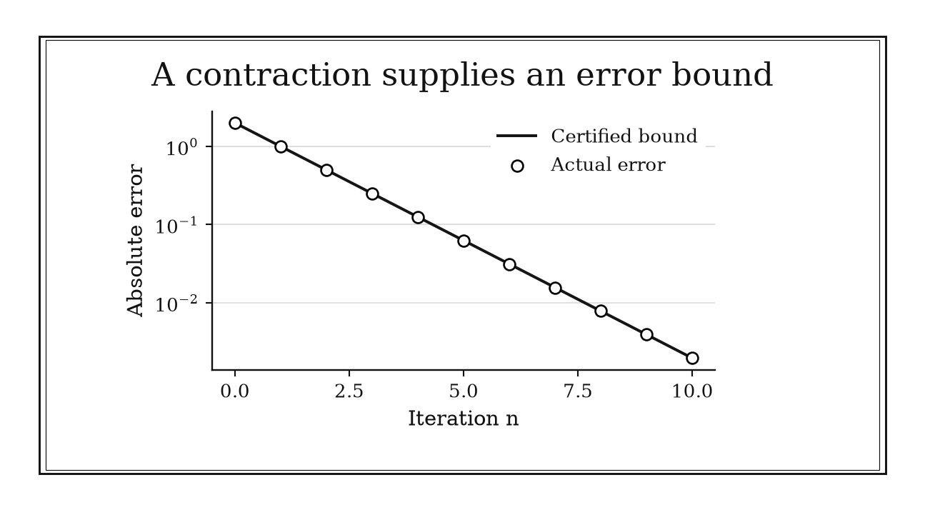
Figure 5.1. Iteration x_next=0.5x+1 from x=0 converges to 2. The contraction bound from the initial step equals the actual error in this constructed linear example; equality is not typical.
5.1.3: Demand uniform control before interchanging limits
History
Cauchy’s 1821 Cours d’analyse makes a plausible claim: a series of continuous functions that converges, settles toward one fixed sum, has a continuous sum. It seems to follow from common sense: if every partial sum is continuous and the sums settle down, why would continuity vanish at the destination? Working in Christiania and Berlin around 1826, Niels Henrik Abel found series that settled down at each fixed point separately yet produced a broken, discontinuous limit overall; checking behavior one point at a time did not supply enough control. The correction crystallized later into a criterion demanding one shared settling rate across the whole domain, isolated after Abel rather than stated by Cauchy himself.
The equation
A sequence converges uniformly to on when
Equivalently, for every there is one such that
How to read it
Convergence checked one input at a time, called pointwise, means the sequence eventually nears the limit at each fixed input, though how soon depends on which input you picked. Uniform convergence, one shared waiting time for every input at once, removes that dependence: the worst gap across the domain, written , short for supremum, must itself shrink toward zero. Uniform convergence preserves continuity and allows term-by-term integration on a finite interval, but it is not a universal license: differentiation through a limit on an interval needs extra hypotheses, such as uniform convergence of the derivatives together with convergence of the function values at one point.
How to use it
A hydrologist models a reservoir’s inflow using forecast curves on , where marks a normalized position along the storm’s timeline. Before integrating the limiting forecast to report total inflow, the hydrologist must check whether the limit can be swapped with the integral at all.
For every fixed , , while for every , so the pointwise limit is Every is continuous but is not, so convergence cannot be uniform: points just below push close to while there, giving for every , never shrinking.
The hydrologist instead looks for a theorem matched to the operation, dominated convergence or a monotone bound rather than uniform convergence, since Rule 5.2.1 supplies a practical test when available. This is a Workflow rule: it prevents an invalid interchange and directs the next proof.
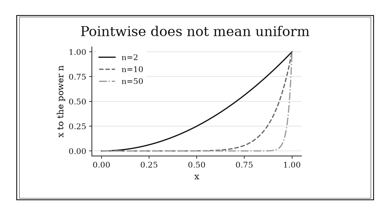
Figure 5.2. On [0,1], x^n tends to zero at every x<1 but remains one at x=1. The limit is discontinuous, and the supremum error remains one; pointwise convergence does not justify a uniform-limit claim.
5.2: Select a Convergence Test That Matches the Evidence
No single convergence test is best. The useful question is what the expression is already offering: a uniform majorant, a tail bound, absolute values, or a recognizable leading term. These four rules turn those clues into a short routing system.
5.2.1: Use the M-test for uniform convergence of function series
History
Proving a series of functions converges is often the easy part; proving it converges uniformly, with one shared settling rate across the whole domain rather than one that drifts point to point, is where arguments stall. During his Berlin lectures in the 1860s, Karl Weierstrass made that distinction central to analysis. The comparison test now bearing his name lowered the stakes. Cover every term with a single numerical ceiling independent of where you evaluate it, then let a convergent number series vouch for the family. Today’s notation was standardized later, but the move survives: one numerical envelope, and every tail inherits its convergence.
The equation
If numbers satisfy
and
then
converges uniformly and absolutely on .
How to read it
Here is a single numerical ceiling covering the size of the th function term everywhere in the domain at once, rather than only at one point. Once such a ceiling exists for every term, and the numbers sum to a finite total, every leftover piece of the series, its tail beyond term , is trapped under the matching leftover of the numerical series. That leftover’s worst-case size across the domain, written , short for supremum, shrinks to zero at the same rate everywhere. The test proves convergence and hands back an error bound together, but it need not reveal what the sum equals.
How to use it
A structural engineer models a beam’s vibration as harmonic terms , where is a damping ratio satisfying . Before certifying the deflection can be integrated term by term, the engineer needs the stronger, uniform kind of convergence, holding across every ratio at once.
Every term satisfies The geometric series converges, so certifies uniform and absolute convergence on . The tail beginning at the tenth term is bounded by small enough to sign off the deflection estimate.
Trying instead gives the divergent harmonic series, proving nothing even though the original series still converges; the fix is a sharper bound, not a verdict against uniform convergence. This is an Independent rule: it directly certifies uniform and absolute convergence and can also return a usable tail ceiling.
5.2.2: Use the Cauchy criterion when the limit is unknown
History
Guessing a series’ destination before proving it converges fails once no destination is obvious. Earlier texts often assumed a suspected sum or geometric target. In his 1821 Cours d’analyse, written in Paris, Augustin-Louis Cauchy reorganized analysis around limits, and later notation distilled his approach into an internal test: measure how late terms sit relative to each other, not relative to an unnamed target. If every pair of sufficiently late terms can be forced arbitrarily close together, the destination need not be named in advance; completeness of the space supplies it.
The equation
A sequence is Cauchy when
In a complete metric space,
How to read it
The criterion trades “where is the sequence going?” for “can its tail still spread apart?” A sequence is Cauchy when, far enough out, every later pair of terms sits closer together than any tolerance you name in advance. Every convergent sequence has this property in any metric space, a space with a defined notion of distance; the substantive direction runs backward: if the space is complete, meaning no Cauchy sequence can head toward a missing point, tail-closeness alone forces convergence.
How to use it
A supply-chain analyst updates a warehouse’s safety-stock estimate weekly using a recursive formula, producing partial totals with no closed-form target in sight. Before committing budget to a fixed reorder point, the analyst needs proof the weekly adjustments are settling down.
Suppose the model guarantees, for every , For a tolerance , choose so : since , works, so totals taken after week differ by less than and the reorder point can be locked in without ever guessing the safety-stock level.
The certificate needs a number system with no gaps, and it is not enough that adjustments merely shrink toward zero: the harmonic terms shrink toward zero while their partial sums drift off without limit. This is a Workflow rule: it turns tail control into an existence proof when the destination is unknown.
5.2.3: Test absolute convergence before conditional behavior
History
A series that only converges through cancellation between positive and negative terms can fall apart the moment its terms are reordered: a fragile kind of success. Cauchy’s 1821 convergence program, worked out in Paris, made that distinction, between cancellation-secured and magnitude-secured convergence, mathematically consequential. Once the terms’ absolute values sum to a finite total, every remaining piece of the series is automatically small, and the stronger conclusion survives reordering in a way conditional convergence cannot. The modern instruction to test absolute convergence first is not Cauchy’s own checklist; it is a method drawn from the theory his program made possible.
The equation
For real or complex terms ,
For every tail,
How to read it
Absolute convergence means the series of magnitudes, every term made positive, adds up to a finite total. When that holds, the original signed series converges automatically, and more strongly: every remaining tail of it is bounded by the matching tail of the magnitude series, an immediate error bound with no extra work. That is sturdier than convergence secured only by cancellation; regrouping and reordering stay safe here, which is not guaranteed otherwise. The implication runs one way only: magnitudes that diverge tell you nothing yet about whether the signs might still rescue the series.
How to use it
A hospital pharmacist is reconciling a running total of alternating dose corrections across a titration schedule, modeled as in normalized units. Before approving that the corrections can be applied in any convenient batch order, the pharmacist checks absolute convergence first.
Taking absolute values, a convergent -series with . The correction series converges absolutely, so the pharmacist can regroup the corrections, batching by shift or patient, without changing the cumulative total.
The same shortcut misleads on a related schedule, : its magnitude series is the divergent harmonic series, so absolute convergence fails, yet the original series still converges conditionally. Reordering that schedule’s corrections is not safe, since a conditionally convergent series can be rearranged to a different total, so the pharmacist keeps those corrections in their original order. This is a Workflow rule: it tries the strongest simple route first and, if that route fails, directs attention to sign-sensitive behavior.
5.2.4: Compare with a model whose threshold you know
History
Two ways to settle whether a series converges pull in different directions: chase an exact closed-form sum, or place the series beside one whose fate is already known. Working in Paris, Cauchy in 1821 sided with the second approach, organizing convergence questions around bounding and comparing tails rather than solving for a sum. The present rule compresses that shift into a recognition habit: strip an unfamiliar positive term down to whatever power, geometric, or log factor controls its size, then compare it with a model series of known threshold.
The equation
For eventually positive sequences and , if
then
either both converge or both diverge.
How to read it
A limiting ratio settling on one positive, finite number says the two sequences differ, in the long run, only by a fixed scale factor. Once confirmed, is eventually trapped between two positive constant multiples of the benchmark , and multiplying a positive series by a fixed constant cannot carry it across the boundary between converging and diverging. Choosing the benchmark is pattern matching: a rational expression built from powers of suggests a -series, terms of the form . The comparison says nothing when that ratio tends to zero or infinity; the test simply does not apply there.
How to use it
A track coach models the cumulative fatigue penalty across a distance race as , where indexes successive laps. The coach wants a quick comparison rather than an exact sum, to answer the idealized question behind the season’s fatigue budget: if the season ran forever, would the total penalty stay finite?
The leading powers suggest the benchmark . Computing the ratio, Because that limit is positive and finite, shares its convergence behavior with , which converges, so the comparison answers the idealized question the budget cap really asks: total fatigue cost stays finite, and the coach plans pacing around it.
The comparison also depends on every staying positive; a tailwind lap recording a negative adjustment would call for comparing absolute values instead. Near a threshold benchmark, keep any log correction rather than dismissing it as “lower order.” This is a Workflow rule: it converts an unfamiliar convergence problem into a familiar model decision.
5.3: Engineer Proofs Instead of Guessing Them
A proof can stall even when the theorem is true. Often the difficulty is architectural: the claim throws away information needed by the next step, the negation preserves the wrong quantifiers, or a local argument lacks a mechanism that prevents escape. These five rules repair the structure before more algebra is attempted.
5.3.1: Extend equality from a dense set by continuity
History
How many points does a continuous function actually need before the rest of its values are no longer up for grabs? Cauchy’s 1821 treatment of continuity, developed in Paris, made the answer sharper than intuition alone would guess. Once a function’s values must track the limits of their inputs, agreement on a sufficiently dense family of points pins down every remaining value. Cauchy did not state the dense-set mnemonic below in that exact form; it packages the rigor he gave continuity. Agreement travels along a sequence of approaching points only because both functions must preserve those limits, turning a partial, checkable fact into a global one.
The equation
Let be dense in a set . If and are continuous on and
then
If is dense in , then .
How to read it
A set is dense in a larger space when every point of that space can be approached as closely as you like by points drawn from the set, even if the set itself is much smaller, the way the rational numbers sit densely among all real numbers. Continuity then forbids two functions from disagreeing anywhere they are both required to track those approaching points. This is a uniqueness principle, not an existence one: it turns a convenient, checkable family into enough evidence for an identity holding everywhere in the closure, all points reachable this way.
How to use it
A municipal water utility models pressure along a supply main with two continuous curves, an existing design curve and a newly fitted curve , confirmed to agree by a continuous-logging survey capable of reading arbitrarily close to any position along the main, an idealization the model adopts explicitly. Before certifying pressure at an unsurveyed address km down the main, the engineer relies on continuity rather than a new sensor.
Choosing surveyed positions approaching , say , each agreeing under both curves, continuity forces certifying the new curve without a sensor.
Both continuity and dense coverage are load-bearing: without continuity, a curve equal to the old design at every surveyed position but redefined elsewhere would satisfy the same agreement while disagreeing almost everywhere, and a survey covering only one short stretch would extend the guarantee no further. This is an Independent rule: its hypotheses directly turn partial equality into a global identity.
5.3.2: Negate quantified claims mechanically
History
Frege’s 1879 Begriffsschrift is a strange-looking artifact: two-dimensional diagrams standing in for what today’s and express in a single row. Frege gave quantified reasoning, generality, nested dependence between variables, implication, and negation, an explicit formal grammar, so a statement could be transformed by manipulating symbols instead of guessing at its failure. Today’s quantifier symbols came later and look nothing like his diagrams, but the legacy survived: negate one operator at a time, from the outside in, and a claim’s failure condition falls out mechanically.
The equation
The two basic transformations are
Thus
How to read it
A universal claim, one asserting something true for every case, fails the moment a single counterexample turns up. An existential claim, one asserting some case works, fails only when every candidate has been tried and fails. When quantifiers are nested, the choices depend on what came before, so their order must survive the negation even as each quantifier flips type. Inequalities must be negated too: a strict bound like , the gap between and a target staying under some small tolerance, becomes , and “ and ” becomes “not or not .” The negation only states the target a counterexample must hit; it neither proves that target exists nor locates the witness.
How to use it
A quality-assurance engineer must write a failure specification for a calibration claim: that a machine’s output sequence settles toward a target as cycles increase, stated as Before the test rig can flag a failing machine, the engineer needs the exact negation.
Negating from the outside inward, each quantifier flips type and the inequality reverses: For a machine oscillating as around , the engineer picks : every cycle count still has some later with , so the rig flags this machine with a reproducible cycle to point to.
Negating only the final inequality while leaving untouched would produce an overly strong failure condition rather than the logical negation. This is a Workflow rule: it creates the exact target for a counterexample or contradiction argument.
5.3.3: Strengthen an induction claim when the step lacks leverage
History
Every course in induction eventually meets a proof that stalls even though the theorem is true, and the standard fix, strengthen the claim, has no textbook origin story. This rule carries an evidence gap: histories of induction are plentiful, but the source search did not turn up a dated episode where someone explicitly repaired a stalled proof by adding the auxiliary fact the next step needed. Later expositions often rewrite an old proof with a stronger invariant built in, crediting the strengthening to whichever mathematician the proof is named for, but without a source dating that move, the credit is retrospective packaging, not a verified event. Closing the gap needs a manuscript showing the failed argument and its repair. Until then, the fair description is a modern proof-design habit, not a dated discovery.
The equation
Replace the desired claim with a stronger claim such that
and prove
The original theorem then follows automatically.
How to read it
Induction is an argument about preserving a pattern: if a statement holds at step and that alone forces it at step , it holds forever once true at the start. When the step stalls, the usual culprit is not that the theorem is too hard, but that the hypothesis is too thin, forgetting information the recurrence needs, the way a relay racer without the baton cannot finish the leg. A useful stronger statement carries exactly the extra context the update step consumes, such as two consecutive bounds instead of one or a parity condition. The new, stronger base case must still be checked and still be true.
How to use it
A bridge inspector certifies a load-capacity bound for a bridge deck built in recursive stages, where the safe load follows with in standardized units, targeting at every stage. The induction step directly stalls: the bound at stage alone does not control the stage- term the recurrence also needs.
Strengthen the claim to a pair, holding at . Assuming it holds at , so the pair carries forward and the certification closes for every stage.
Had the inspector added a condition failing at stage , the certification would rest on a first step that was never actually checked. This is a Workflow rule: it repairs the information flow inside an induction proof.
5.3.4: Use compactness as the signal that escape is impossible
History
An optimization search is only as good as its promise that a best answer exists somewhere inside the search space; without that promise, a search can chase an ever-improving value forever without reaching one. Compactness, the property that makes the promise good, accumulated across the nineteenth century: Bernard Bolzano, in Prague, proved an early version of the fact that a bounded sequence must have a subsequence that settles down; Karl Weierstrass, in Berlin, made such accumulation arguments central to rigorous analysis; and Emile Borel, later in Paris, formulated the finite-covering property for closed bounded intervals. The modern definition anchors on their combined results; the summary phrase is later teaching shorthand.
The equation
In finite-dimensional Euclidean space,
Consequently,
and, when is nonempty, every continuous attains both a minimum and a maximum.
How to read it
A set is bounded when it fits inside some fixed finite region, and closed when it contains every point its own members can approach, leaving no gap to escape through. In finite-dimensional space, having both properties at once is what compact means. Boundedness stops a wandering sequence from drifting to infinity; closedness stops it from sneaking out through a missing boundary point. Together, every sequence inside a compact set has a subsequence, an ordered selection of its terms, that settles down to a limit still inside the set, and every continuous function on it reaches its highest and lowest values. Outside finite dimensions, closed and bounded no longer guarantee compactness, and even when a maximum exists, the rule never says where it occurs.
How to use it
An environmental monitoring station reports pollutant concentration as a continuous function of time of day, in normalized units, over a reporting window, and regulators need to certify that a single worst-case reading actually occurs, rather than a ceiling concentrations only approach.
Over the closed window , compactness guarantees attains its maximum, , at the window’s closing instant, so the station certifies a specific, timestamped reading.
Suppose instead the window is open, , excluding its boundary instants. The same function then has supremum, the least upper bound, of but no reading that attains it: climbs toward without arriving, since for every , so a report claiming a worst-case value of would certify a reading that never happened. This is a Workflow rule: compactness supplies the existence mechanism inside optimization, convergence, and subsequence arguments.
5.3.5: Choose delta by working backward from epsilon
History
Guessing a workable delta by trial and error wastes effort and rarely generalizes. In Paris, Cauchy’s 1821 limit framework required an error to become arbitrarily small before a limit could be declared, though the explicit epsilon-delta symbolism used today was refined later in the nineteenth century, moving from infinitesimal language toward checkable inequalities. This rule is a modern proof-writing method built on that refinement, not a phrase Cauchy wrote. Delta is not guessed from the input side. The proof writer starts from the demanded output error, reverses the algebra, and reads off a sufficient input restriction.
The equation
To prove
whenever , seek a local bound
Then it is sufficient to choose
How to read it
An epsilon-delta proof is an implication running one direction: if the input stays within an allowed distance of a target, the output stays within a demanded tolerance of its own target. Working backward: start from the tolerance you must hit, trace the algebra back to the input distance, and discover how small a restriction forces it. The final proof runs forward instead: assume the restriction, apply the bound, and land inside the tolerance. If the controlling constant depends on where the input sits, impose a simple local restriction first, so it becomes one fixed number.
How to use it
A logistics analyst models estimated fuel cost for a return trip as , the planned one-way distance in tens of kilometers, and must guarantee the estimate stays within tolerance of the target cost at planned distance , whenever the actual distance stays within margin of the plan.
Factor the error: Requiring forces , so and . Choosing guarantees whenever . For , : the driven distance may vary by up to forty meters from the plan.
The constant 5 depends on where the plan sits: reusing at a longer planned distance, where exceeds 5, would silently overshoot the tolerance, and dropping the restriction breaks that bound of 5 entirely. A more complicated cost model could pull directly from the Lipschitz bound of Rule 5.1.1. This is a Specialized rule: it is a highly reliable construction inside epsilon-delta limit and continuity proofs rather than a standalone numerical answer.
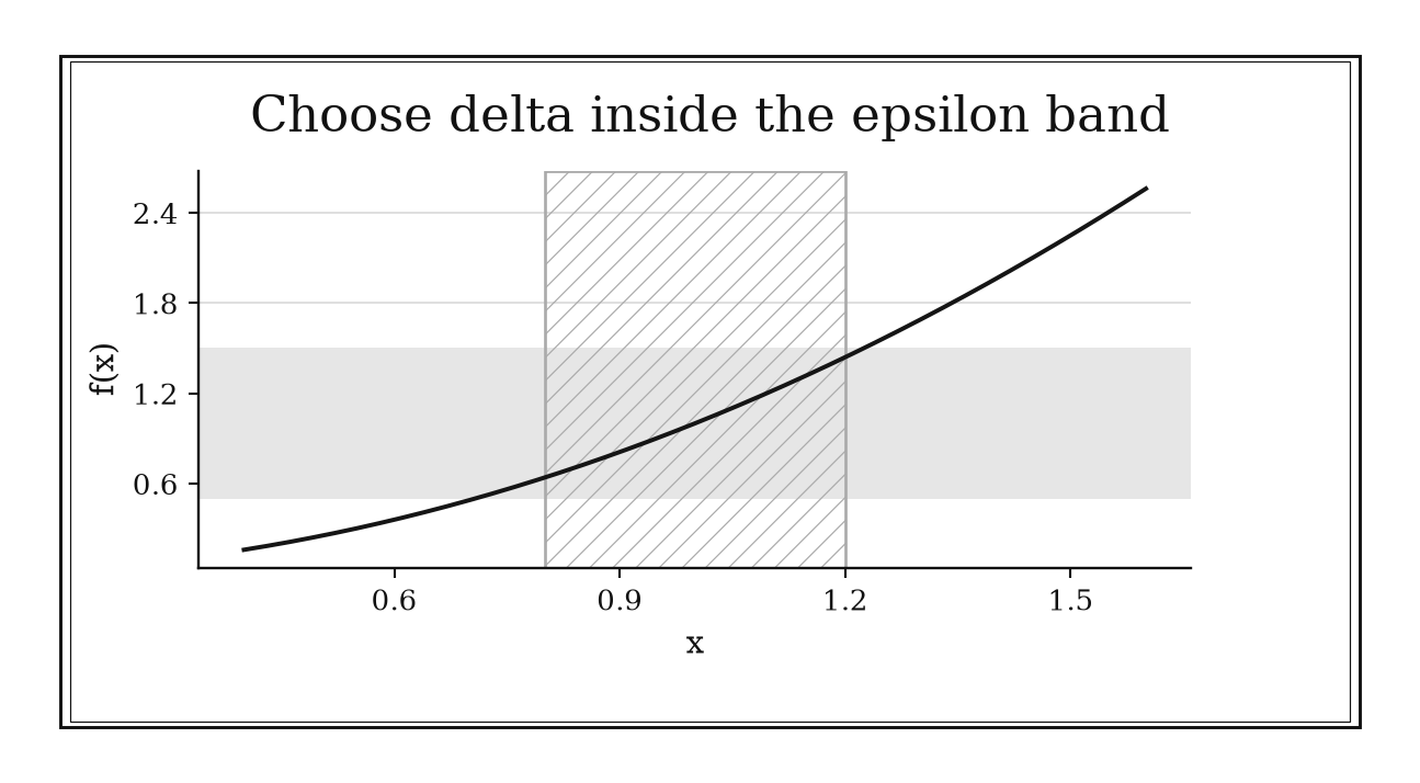
Figure 5.3. For f(x)=x² at x=1, epsilon=0.5 and delta=0.2 work: |x-1|<0.2 implies |x²-1|<0.44<0.5. The shaded input strip stays inside the output tolerance band.
Chapter Synthesis: Control Before Passage
Analysis earns its reputation for rigor by refusing to let a limiting operation hide its assumptions. The practical version of that rigor is not a longer proof every time. It is a short set of control questions asked early.
First quantify sensitivity. A Lipschitz constant converts input error into output error, while a contraction constant converts a completed step into remaining fixed-point error. Then ask whether the control is pointwise or uniform. A statement that succeeds separately at every fixed point may still fail when a bad region moves with the index.
For convergence, use the evidence already present. A uniform numerical majorant suggests the M-test. A direct tail estimate suggests the Cauchy criterion. Sign changes suggest testing absolute convergence before studying cancellation. A recognizable dominant term suggests comparison with a benchmark sequence.
For proofs, make the logical structure visible. Continuity transports equality from a dense set. Quantifier negation defines exactly what a counterexample must do. A stronger induction invariant restores information the recurrence needs. Compactness prevents candidates from escaping. Backward epsilon-delta algebra turns a desired accuracy into a sufficient input restriction.
Across all twelve rules, ask four questions:
- What quantity is being controlled?
- Is the control local, pointwise, uniform, or global?
- What property of the space makes the conclusion exist inside it?
- Does the rule finish the argument, or prepare the theorem that will?
One-Page Analysis Toolkit
| Recognition cue | Rule to try | What it gives | Role |
|---|---|---|---|
| Input uncertainty enters a regular map | Bound it with a Lipschitz constant | Output-error ceiling | Independent |
| Fixed-point iteration has verified rate | Multiply the last step by | Remaining-error bound | Workflow |
| A limit is about to cross another operation | Test for uniform or theorem-specific control | Interchange guardrail | Workflow |
| Function terms have point-independent bounds | Apply the M-test | Uniform and absolute convergence | Independent |
| A limit is unknown but tails can be bounded | Use the Cauchy criterion | Convergence without a guessed destination | Workflow |
| A series changes sign | Test absolute values first | Strong convergence route or routing result | Workflow |
| A positive tail resembles a known model | Use limit comparison | Shared convergence behavior | Workflow |
| Continuous functions agree on a dense family | Pass equality through limits | Global identity | Independent |
| A theorem’s failure must be stated | Negate quantifiers outside-in | Exact counterexample target | Workflow |
| An induction step lacks needed context | Strengthen the invariant | A closable induction step | Workflow |
| Candidates may approach infinity or a missing boundary | Look for compactness | Extrema or convergent subsequences | Workflow |
| An epsilon-delta proof feels like guessing | Work backward from epsilon | Constructive delta choice | Specialized |
Decision Path
- Is the problem about perturbation or numerical error? Find a Lipschitz or derivative bound. If an iteration is a verified contraction, translate its last step into a stopping certificate.
- Are functions converging? Before moving a limit through continuity, integration, differentiation, or summation, name the governing interchange theorem. Check whether its control is uniform and whether one bound works across the entire domain.
- Is the object a function series? Seek a point-independent majorant and try the M-test.
- Is the limit unknown? Compare late terms or partial sums with one another. A tail estimate plus completeness may be enough.
- Does a numerical series change sign? Test absolute convergence first. If that fails, move to cancellation-sensitive tests.
- Does a positive term have a recognizable leading scale? Compare it with a -series, geometric series, or logarithmic benchmark.
- Is a proof stalled? Inspect its architecture: use density plus continuity for identity, formal negation for counterexamples, a stronger invariant for induction, compactness for existence, or backward error algebra for epsilon-delta construction.
Transfer Problems
1. Build an error certificate
An iteration is known to be a contraction with . Its latest completed step has size . Bound the remaining error. Then suppose the final quantity is passed through a function with Lipschitz constant . Bound the resulting output error and decide whether a tolerance of is certified.
2. Route the convergence evidence
For each object, identify the first test you would try and state the hypothesis that must be checked:
Do not compute a closed-form sum. The task is to choose and justify the shortest valid convergence route.
3. Repair the proof before finishing it
Someone claims that a continuous function on must attain its maximum because the interval is bounded. Identify the missing compactness condition and give a counterexample. Then write the quantified negation of “ attains a maximum on its domain.” Finally, state what changes if the domain is replaced by .
Where These Ideas Reappear
- Calculus: derivative bounds become Lipschitz estimates, while Taylor remainders make local approximation errors explicit.
- Complex analysis: uniform convergence and compact subsets control function series, differentiation, and contour arguments.
- Linear algebra: operator norms act as error amplifiers, contraction-like spectral rates control iterations, and completeness supports convergence.
- Probability and statistics: dominated convergence governs limit-expectation interchange; concentration bounds turn random error into quantified tails.
- Optimization: compact feasible sets yield minimizers, Lipschitz constants set step sizes, and contraction estimates certify fixed-point algorithms.
- Numerical methods: Cauchy-style tail bounds, a posteriori error estimates, and stopping criteria separate observed progress from certified accuracy.
- Topology and functional analysis: compactness and completeness retain their roles, while “closed plus bounded” must be replaced by space-appropriate criteria.
Historical Notes and Sources
The historical profiles distinguish documented events from modern operational interpretations. The induction-strengthening profile remains an explicit evidence gap rather than receiving an invented origin story.
- Lipschitz and controlled variation: MacTutor biography of Rudolf Lipschitz.
- Banach’s contraction principle: Centenary historical study of Banach’s fixed-point theorem.
- Cauchy’s 1821 convergence program: Bibliothèque nationale de France record for Cours d’analyse; MacTutor biography of Augustin-Louis Cauchy.
- Abel and the correction of overbroad convergence claims: MacTutor biography of Niels Henrik Abel.
- Weierstrass and uniform convergence: MacTutor biography of Karl Weierstrass.
- Frege and formal quantification: Göttingen digitization of Frege’s Begriffsschrift; Frege.info scholarly project.
- Bolzano, Weierstrass, Borel, and compactness mechanisms: MacTutor biography of Bernard Bolzano; MacTutor biography of Émile Borel.
- Mathematical statements and proof conventions: Jiří Lebl, Basic Analysis: Introduction to Real Analysis; MIT OpenCourseWare real analysis notes; MIT OpenCourseWare, Mathematics for Computer Science.