Chapter 6: Complex Analysis: Turn Analytic Structure into Bounds and Counts
For a nonconstant function analytic in a bounded domain and continuous on its closure, the largest modulus is found at the boundary, not at an interior point. That result feels surprising only if the function is treated as an arbitrary surface over the plane. Analyticity ties its interior behavior so tightly to its boundary values that the boundary can control derivatives, integrals, extrema, and even the number of hidden zeros.
Complex analysis rewards the right first move. Products want polar form. Logarithms demand a declared branch. Candidate analytic functions should be screened before analytic theorems are used. Contour integrals often need a bound or a residue calculation rather than direct parameterization. Root questions may be settled by comparing boundary magnitudes instead of solving for any root.
The ten rules in this chapter follow that progression. The first three choose a representation and test whether analytic structure is present. The next three turn analyticity into immediate bounds. The final four use local singular behavior or boundary winding to evaluate integrals and count zeros. Five can directly answer a question; five are compact steps inside a larger contour workflow.
The governing habit is: identify the representation, branch, contour, and analyticity assumptions before invoking the power of the complex plane.
6.1: Choose a Representation That Exposes Structure
A complex number carries both magnitude and direction. Cartesian form exposes addition, while polar form exposes multiplication. Before manipulating an expression, decide which structure matters and whether the function is single-valued and analytic on the region being used.
6.1.1: Use polar form for complex products and powers
History
A memoir on directed line segments, presented to the Royal Danish Academy in Copenhagen in 1797 and published in 1799, gave Caspar Wessel’s answer to multiplying two arrows instead of two numbers. He described each segment by its length and its direction, and showed that multiplying two segments meant multiplying the lengths and adding the directions. Modern exponential notation and the classroom polar-form routine came later; the geometric split is his. The rule keeps that split: when the operation is multiplication or a power, separate size from direction first.
The equation
Write two nonzero complex numbers as
where , , and the angles are arguments. Then
For an integer ,
The magnitudes multiply while the arguments add. Taking a power repeats both operations: raise the magnitude to the power and multiply the angle by it.
How to read it
Every nonzero complex number is fixed by two numbers: how far it sits from zero (its magnitude) and which way it points (its angle, or argument). Multiplying two complex numbers multiplies their magnitudes and adds their angles; raising one to a whole-number power raises the magnitude to that power and multiplies the angle by it. That gives a free check: the answer’s distance from zero is the product of the two distances, and its direction matches the sum of the two directions, full turns aside. The shortcut favors multiplication and powers; for addition, plain coordinates stay simpler.
How to use it
A field surveyor runs a staked point through eight identical correction steps, each multiplying its complex map coordinate by . Rather than multiply real and imaginary parts eight times over, the surveyor switches to polar form. Since and its angle is ,
The chain scales the plotted distance by and, since eight eighth-turns make one full turn, returns the bearing in line with the original. Reading the angle as a raw radian count instead of modulo one full turn would make the chain look like it added a bearing offset, sending a field crew chasing a turn that does not exist. This is an Independent rule: once a nonzero complex product or integer power is recognized, polar form can deliver the result directly and supply separate magnitude and phase checks.
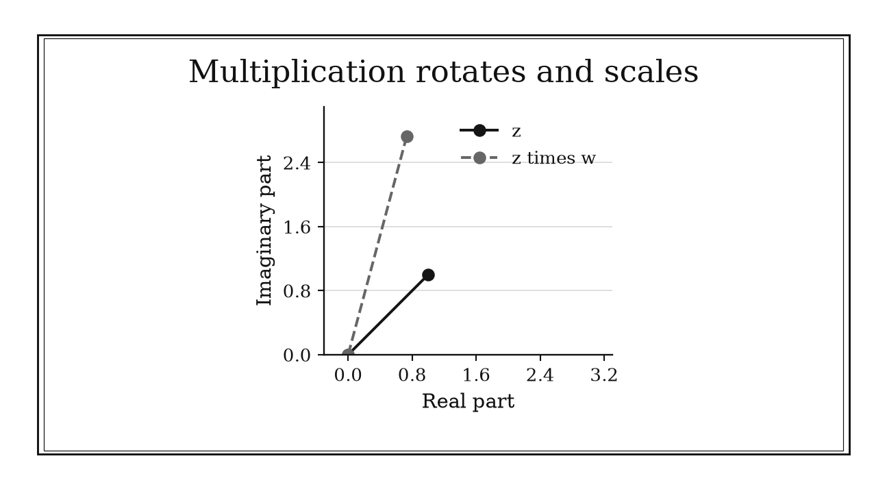
Figure 6.1. Multiplying z=1+i by w=2 exp(i pi/6) doubles the distance from the origin and adds 30 degrees to the argument. Magnitudes multiply; angles add modulo a full turn.
6.1.2: Treat the principal argument as branch-dependent
History
A complex logarithm can silently swap one valid value for another, with no warning built into the arithmetic, whenever the branch goes unstated. During the 1740s, Euler and d’Alembert exchanged arguments from Berlin and Paris about the logarithm of a negative or complex number, exposing a genuine difficulty: a complex logarithm cannot be made single-valued everywhere without an explicit choice, a point Euler’s later systematic treatment of exponentials and trigonometric functions left unresolved. The principal argument, one chosen angle out of infinitely many that describe the same direction, is the modern convention for fixing that choice; the debate is what made the choice necessary.
The equation
For , a common principal-value convention is
The interval selects one representative angle and assigns for , but the resulting principal value is discontinuous across the negative real axis. When is needed as an analytic branch, use the slit domain and . Zero and the cut are then excluded from the branch domain.
How to read it
A complex number’s argument is simply the angle it makes as an arrow from zero; the principal argument picks one such angle, conventionally between and , as the standard choice. The complex logarithm pairs an ordinary logarithm of distance from zero with that chosen angle. A branch cut is a boundary line, here the negative real axis, sliced out of the domain so a continuously tracked angle never has to jump anywhere else. Cross that line and the recorded angle jumps by nearly a full turn, even though the number itself changes smoothly. The convention fixes one value; the other equally valid values do not disappear.
How to use it
A filter designer traces the phase of a transfer function as frequency sweeps a curve passing close to , once from just above the negative real axis and once from below. Approaching from above, the principal argument climbs toward ; from below, it sinks toward . The two principal logarithms on either side of differ by , though the underlying values sit close together and change continuously. Feeding both into without checking which side of the cut each sits on makes the sweep disagree by a stray , showing a phase jump no physical filter produces. Declaring which branch is in use before combining logarithms removes that false jump. This is a Workflow rule: a branch declaration does not finish most complex-logarithm problems, but it prevents a locally valid simplification from becoming globally false.
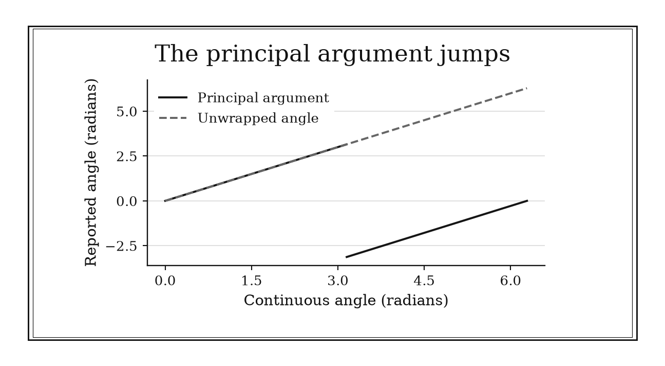
Figure 6.2. As a point crosses the negative real axis, its continuous rotation passes pi while the principal argument wraps to -pi. The jump belongs to the branch convention, not to the point’s motion.
6.1.3: Use Cauchy-Riemann equations as a quick analyticity screen
History
A proposed potential-and-stream-function pair can look smooth and reasonable on paper yet fail to define an analytic complex potential. In 1752, studying fluid motion in Paris, d’Alembert wrote down relations between pairs of functions that expose exactly that failure; they are now known as the Cauchy–Riemann equations, and Cauchy and later Riemann made them central to complex differentiability, the property a function must have to be called analytic. Using a failed relation as a rapid rejection test is a modern diagnostic; passing it at one point is not, by itself, a license to use every theorem of complex analysis nearby.
The equation
Write
Complex differentiability requires
When the first partial derivatives are continuous in a neighborhood, satisfying these relations there gives the regularity needed for the standard analyticity conclusion.
How to read it
Write a complex function as a pair of real functions, and , for the real and imaginary parts of the output. Being complex differentiable at a point means the rate of change comes out the same however the input is nudged. Comparing a horizontal nudge to a vertical one forces two matching conditions on the partial derivatives: one pair must agree, the other must be exact opposites. If either fails at a point, the function cannot be complex differentiable there. Passing both at a single point is weaker: it does not certify analyticity throughout a neighborhood, and the usual regularity assumptions still have to hold.
How to use it
A fluid-dynamics engineer checks a proposed complex potential , with proposed as its potential and as its conjugate stream function. The question is whether this particular pair defines an analytic complex potential. Computing the needed partial derivatives gives
so fails everywhere, since : the candidate model is nowhere complex differentiable, and this proposed potential-and-stream-function pair cannot be used as an analytic complex potential. Checking the relation at a single grid point, without scanning the rest of the domain, could instead wave through a model that fails everywhere else nearby. Running the screen across the whole candidate domain avoids that mistake. This is a Workflow rule: the screen rapidly rejects nonanalytic candidates and routes valid candidates toward analytic tools, but it is usually a qualification step rather than the final answer.
6.2: Convert Analyticity into Immediate Bounds
Once analyticity has been established on the required region, a contour’s length, radius, and boundary magnitude can control much more than the boundary itself. These rules replace difficult evaluations with certified ceilings and boundary checks.
6.2.1: Bound a contour integral by maximum times length
History
A contour integral, one totaled along a chosen path through the complex plane, can be shown to vanish in a limit without ever being evaluated exactly, simply by bounding it from above. That traces to Cauchy’s memoirs on definite integrals with imaginary limits, written in Paris between 1825 and 1831, which developed contour-deformation ideas and what he called residues, a systematic way to connect such an integral to the singular behavior it encloses. The maximum-times-length estimate is a compact modern consequence: a certified ceiling built from nothing more than the largest integrand value on the path and the path’s length.
The equation
For a rectifiable path and a function continuous on its image,
The right side is commonly remembered as : an integrand-magnitude ceiling multiplied by path length .
How to read it
The size, or modulus, of a contour integral cannot exceed the largest value the integrand’s modulus takes on the path, times the path’s length, like a delivery bill capped by the highest per-mile rate times the miles driven. Cancellation can make the true integral much smaller; the bound only promises it will not be larger. This separates two jobs: measure the path’s length once, bound the integrand’s size once, and multiply. A single overall maximum can still be too generous when the integrand varies sharply across the path.
How to use it
An actuary is closing a transform-inversion contour with a large circle of radius , a standard step in recovering a loss distribution from its transform, and needs to know whether the circle’s contribution can be ignored as grows. On the integrand is , so
As grows, that ceiling shrinks to zero, so the actuary discards the circle, keeping only the contributions from the poles, where the transform blows up, inside the path. One crude bound would mislead if the function’s magnitude varied sharply across the circle; splitting it into arcs with separate bounds avoids that. This is an Independent rule: when only a certified magnitude ceiling or a vanishing contribution is needed, the estimate can answer the question without evaluating the contour integral.
6.2.2: Use Cauchy’s estimate to bound derivative scale
History
A function that is analytic, meaning complex differentiable throughout a region, might seem free to change arbitrarily fast at one point while staying small everywhere nearby, the way a plucked string could jitter faster without its amplitude growing. Between 1825 and 1831, Cauchy’s Paris memoirs on definite integrals with imaginary limits said otherwise: by 1831 his work tied a contour integral to the local singular behavior it encloses. Cauchy’s derivative estimate, drawn later from that framework, converts a boundary size bound and a chosen radius into a hard ceiling on every derivative at the center, closing off the fast-wiggle possibility for any genuinely analytic function.
The equation
If is analytic on an open set containing the closed disk and
on that circle, then for every integer ,
The reflects differentiation, while each derivative costs another factor of inverse radius.
How to read it
The th derivative at the center of a disk measures how sharply the function curves there; larger means a higher-order rate of change. That derivative cannot exceed () times the largest value on the surrounding circle, divided by the circle’s radius raised to the th power. A bigger radius, meaning more room before the nearest obstruction, pushes the ceiling down; a nearby singularity forces a small radius and removes that leverage. The bound is guaranteed, not a claim that any actual derivative gets close to it.
How to use it
A vibration engineer models a damped structure’s frequency response as an analytic function and has confirmed on , where the radius represents how far the model is trusted from resonance. Taking and ,
Both ceilings follow without differentiation once analyticity throughout the closed disk is verified. If a singularity lies within radius , the choice is invalid and the value is no longer certified. The engineer chooses a radius strictly smaller than the distance to the nearest singularity, re-verifies on the new circle, and recomputes both ceilings before trusting the model. This is an Independent rule: given a verified analytic disk and boundary bound, Cauchy’s estimate directly supplies a derivative or Taylor-coefficient ceiling.
6.2.3: Look on the boundary for analytic maxima
History
Does checking a function’s size everywhere inside a region ever reduce to checking it only on the edge? Cauchy’s contour program, developed in Paris between 1825 and 1831, says yes for analytic functions, ones that are complex differentiable throughout the region: his memoirs tied a contour’s boundary data to the singular behavior sealed inside it. The maximum-modulus principle states the sharpest version, reached later: a nonconstant analytic function on a bounded region cannot reach its largest modulus, its greatest distance from zero, at an interior point, so the search can move entirely to the boundary.
The equation
If is analytic in a bounded domain and continuous on its compact closure , then
If the maximum occurs at an interior point, the analytic function must be constant on the relevant connected domain.
How to read it
The modulus of a complex number is its distance from zero, the size of the arrow representing it. For a function analytic throughout a region and continuous up to its edge, the largest modulus anywhere in the region, interior included, always turns up on that edge, never strictly inside. That collapses a search over a whole two-dimensional area to a search along the boundary curve. The principle covers maxima only; it cannot certify the smallest modulus, since an analytic function can equal zero deep inside.
How to use it
A vibration engineer models a complex response on a circular plate as and needs the largest can reach on the disk representing the plate’s radius. Checking only the rim :
with equality when , so the largest modulus over the entire plate is , found without evaluating a single interior point. Reporting that as the largest modeled response amplitude is valid only because the model is analytic inside the disk and continuous to its edge; a hidden interior singularity would make the shortcut meaningless. The principle gives no help for the plate’s smallest response amplitude, since an analytic function can dip to zero well inside. This is an Independent rule: under the analytic and compactness hypotheses, the boundary search directly determines or bounds the maximum modulus over the whole region.
6.3: Turn Singularities and Boundary Behavior into Counts
Analytic functions store global information in local singular coefficients and in the way their boundary values wind around zero. The four rules here are a routing system: identify pole structure, convert residues into integrals, or compare boundary behavior to count unseen zeros.
6.3.1: Compute a simple-pole residue by division of derivatives
History
A short division, numerator over denominator derivative, is the entire tool this rule packages, descended from Cauchy’s memoirs on definite integrals with imaginary limits, written in Paris from 1825 through 1831. Those memoirs developed contour-deformation ideas and what Cauchy called residues, numbers capturing how a function behaves near a singular point, tying a contour integral, a path integral through the complex plane, to that behavior. That residue calculus later gave the derivative-division shortcut: for a quotient whose denominator has a simple zero, it extracts the one number a contour integral needs, without constructing the full local series expansion.
The equation
Let and be analytic near , and let
If
and , then is a simple pole and
The nonzero derivative confirms that the denominator zero is simple.
How to read it
Near a point where the denominator of a quotient hits zero just once, called a simple pole, that denominator behaves almost like a straight line through zero, with slope equal to its derivative there:
Dividing the numerator’s value by that slope gives a number called the residue, the coefficient of that would appear in the full local series expansion, the Laurent series, around that point. If the denominator’s zero repeats, then and a higher-order analysis is needed. If but the numerator also vanishes, the singularity is removable and the same residue quotient gives zero.
How to use it
A circuit designer decomposes a system’s response
into terms, one per pole, and needs the term for the pole at . Writing and , so , the residue is
That number becomes the coefficient of this pole’s term in the system’s response, computed without expanding any series. The designer checks the numerator does not also vanish at ; if were zero too, the pole would cancel out and the residue quotient would equal zero. The designer also confirms , since a repeated zero would need a higher-order formula. This is a Workflow rule: the quotient formula computes one local ingredient quickly; a larger contour calculation must still identify which poles matter and how their residues are used.
6.3.2: Turn a contour integral into a sum of enclosed residues
History
Walking an entire closed contour by hand is labor a mathematician can skip once the enclosed singularities are known. Between 1825 and 1831, Cauchy’s Paris memoirs on definite integrals with imaginary limits developed contour-deformation ideas and residues, the local numbers a function leaves at its singular points, into a systematic method. The decisive shift was from tracking every path point to extracting local information from enclosed singularities; the modern workflow locates the poles, where a function blows up, and sums their coefficients instead of walking the path.
The equation
Let be a positively oriented, simple, closed, piecewise-smooth contour. If is meromorphic on an open set containing and its interior, with poles inside and no poles on , then
Reversing the contour orientation reverses the sign of the integral.
How to read it
A function is meromorphic in a region if it behaves smoothly, complex differentiable, everywhere there except at a handful of isolated blow-up points called poles. Its integral around a closed path, or contour, enclosing some of those poles equals times the sum of the residues, the local numbers each enclosed pole contributes. What remains after removing those contributions behaves well enough that its own loop integral vanishes. Tracing the path the other way flips the sign of the integral, and a pole outside it, however large its residue, contributes nothing.
How to use it
A signals engineer needs the value of
that shows up while inverting a filter’s transfer function around the unit circle. The integrand has poles at and , but only lies inside ; the pole at sits outside and drops out. The residue at is
The engineer reports that value without parameterizing the circle. The standard way this goes wrong is including a pole that sits outside, like , or missing one on rather than strictly inside. When the contour only evaluates a real integral, the engineer must confirm any auxiliary arc vanishes, typically via a maximum-times-length bound. This is a Workflow rule: the theorem replaces contour integration with a finite residue sum, but contour choice, pole classification, and auxiliary-bound checks remain parts of the larger method.
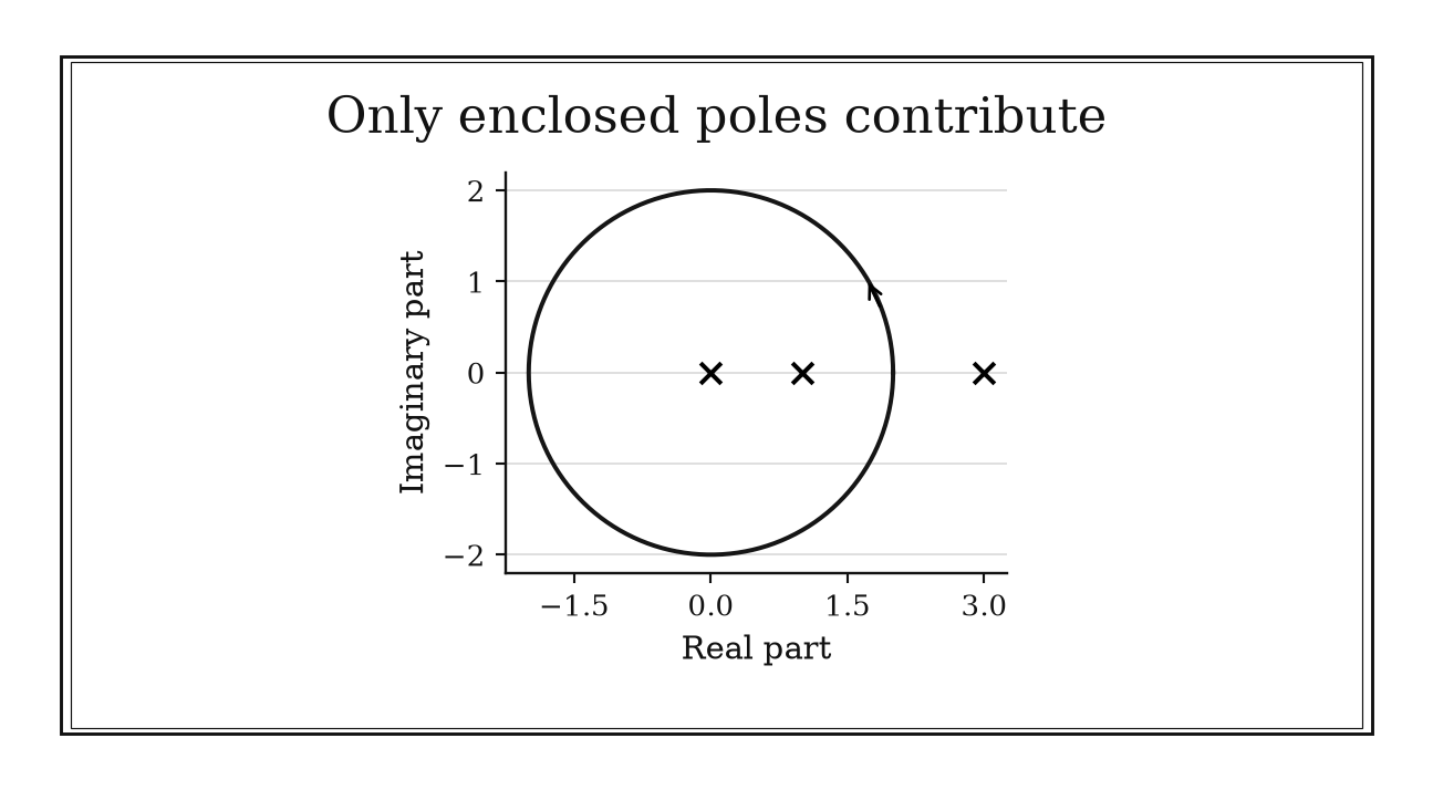
Figure 6.3. For a positively oriented circle of radius two, the poles at 0 and 1 are enclosed while the pole at 3 is excluded. With unit residues, the contour integral is 2pi i times two.
6.3.3: Use Rouché when one boundary term dominates
History
Solving directly for every zero, every point where a function equals zero, of a complicated expression can be hopeless when only the count is needed, not the locations. In 1862 in Paris, Eugène Rouché published a theorem for exactly that difficulty, in a memoir on Lagrange’s series: if one analytic term dominates another in size everywhere along a closed contour, a path through the complex plane, adding the smaller term to the dominant one does not change how many zeros sit inside. Rouché’s theorem is the historical result; the present rule splits a difficult function into an easy dominant part and a smaller, controllable perturbation.
The equation
Let be a simple closed contour. If and are analytic on an open set containing and its interior, and
then and have the same number of zeros inside , counted with multiplicity.
How to read it
A zero of a function is a point where it evaluates to . Rouché’s comparison says that if one analytic piece, , has a strictly larger modulus, a greater distance from zero, than another piece at every contour point, then alone and enclose the same number of zeros inside, counted with repetition. The two need not have zeros anywhere close together; only the total count must match. The comparison is a certificate, not an impression: must hold at every point on the contour, not on average.
How to use it
A systems modeler uses the complex polynomial as a response model and asks whether the correction changes its number of zeros inside . Splitting the corrected polynomial as
the designer checks both terms on that circle:
Since on , the corrected polynomial keeps the same five enclosed zeros as , counted with multiplicity. Their positions can change; this count alone does not locate a physical response null. Had the correction been large enough to violate there, the comparison would certify nothing, and the modeler would need a different contour or split. This is an Independent rule: once strict boundary dominance is certified, Rouché’s theorem directly answers the enclosed zero-count question without solving for the zeros.
6.3.4: Count zeros minus poles with the argument principle
History
Counting a function’s zeros and poles, where it blows up, can come down to one contour integral that keeps a running ledger: zeros add, poles subtract, and multiplicity, how many times each repeats, sets the weight. That ledger follows from Cauchy’s contour and residue work, carried out in Paris between 1825 and 1831, connecting a boundary integral to the singular behavior inside it. The argument principle, distilled from that connection, is built around a function’s logarithmic derivative, turning its residues into that ledger of zeros minus poles.
The equation
Let be a positively oriented, simple, closed, piecewise-smooth contour. If is meromorphic on an open set containing and its interior and has no zeros or poles on , then
where and count enclosed zeros and poles with multiplicity.
How to read it
The logarithmic derivative of a function is its ordinary derivative divided by the function itself, . Near a zero of order , meaning it behaves like there, this ratio contributes a local number, its residue, equal to ; near a pole of order , where the function blows up, it contributes instead. Adding those contributions inside a contour gives enclosed zeros minus poles, weighted by order, or multiplicity. The same integral counts how many times the boundary values wind around zero, so a zero or pole on the path breaks the method.
How to use it
A suspension-control engineer uses the polynomial as a contour-count check on . Its polynomial form rules out poles, and the logarithmic derivative is
The zeros of are the three roots of , each of modulus , so : the integral counts the three enclosed zeros because the polynomial is already known to have no poles. This count on alone does not certify system stability. The engineer first checks no zero or pole sits exactly on : a boundary root does worse than shift the count, it makes the integral itself meaningless. If the winding is measured from sampled data instead, too coarse a sample can miss a phase swing, hiding a root a finer sweep would catch. This is a Workflow rule: the logarithmic-derivative integral is a powerful counting component, but contour validation, pole accounting, and reliable boundary evaluation remain essential parts of the workflow.
Chapter Synthesis: Let the Boundary Do the Work
Complex analysis becomes practical when representation and hypotheses are chosen before computation. Polar form turns products into magnitude multiplication and angle addition. A branch declaration prevents complex logarithms and fractional powers from silently changing value. The Cauchy–Riemann equations reject functions that do not qualify for analytic methods.
Once analyticity is secure, boundary information becomes an engine. Maximum times length bounds a contour integral. Cauchy’s estimate turns boundary size and radius into derivative scale. The maximum-modulus principle reduces an interior search to the boundary.
Singularities and winding complete the picture. A simple denominator zero yields its residue by one derivative. The residue theorem replaces a closed-contour integral by a finite sum. Rouché transfers an easy zero count across a strict boundary perturbation, while the argument principle counts zeros minus poles through the logarithmic derivative.
Across all ten rules, ask four questions:
- Which representation exposes the operation, Cartesian, polar, or logarithmic?
- What branch, contour, and analyticity region has actually been declared?
- Can a boundary magnitude, radius, or winding settle the question?
- Does the result answer the question, or supply one component of a contour workflow?
One-Page Complex Analysis Toolkit
| Recognition cue | Rule to try | What it gives | Role |
|---|---|---|---|
| Product or integer power of nonzero complex numbers | Use polar form | Magnitude and phase result | Independent |
| Complex logarithm, root, or fractional power | Declare the argument branch | Branch-safe interpretation | Workflow |
| Candidate analytic function in form | Check Cauchy–Riemann | Fast rejection or qualification route | Workflow |
| Need only a contour-integral ceiling | Maximum magnitude times path length | Guaranteed upper bound | Independent |
| Analytic disk with boundary bound | Apply Cauchy’s estimate | Derivative or coefficient ceiling | Independent |
| Need a maximum modulus on a compact region | Search the boundary | Global maximum or bound | Independent |
| Quotient with a simple denominator zero | Divide numerator value by denominator derivative | Local residue, zero after cancellation | Workflow |
| Closed contour with isolated enclosed poles | Sum the enclosed residues | Contour integral | Workflow |
| One analytic term strictly dominates on the boundary | Apply Rouché | Enclosed zero count | Independent |
| Boundary evaluation is manageable but roots are hidden | Integrate | Zeros minus poles | Workflow |
Decision Path
- Is the main operation multiplication or exponentiation? Move to polar form. If a logarithm, root, or fractional power appears, state the branch before simplifying.
- Are you about to invoke an analytic theorem? Write , screen with Cauchy–Riemann, and verify the required neighborhood and regularity.
- Do you need a bound rather than an exact integral? Estimate maximum integrand magnitude and contour length. Split the path if one maximum is too crude.
- Do you know a boundary magnitude on an analytic disk? Use Cauchy’s estimate for derivatives; use the maximum-modulus principle for the function’s largest modulus.
- Does a quotient have simple poles? Compute each needed residue by numerator value over denominator derivative.
- Is the contour integral closed? List and classify enclosed poles, check orientation, and use the residue theorem.
- Is the real question a zero count? Try Rouché when one term dominates on the boundary. Use the argument principle when or boundary winding is more accessible.
Transfer Problems
1. Separate magnitude, phase, and branch
Write in polar form and evaluate without repeated Cartesian multiplication. Then compare the principal arguments obtained when a point approaches the negative real axis from above and below. State which part of the work gives a number and which part is a branch guardrail.
2. Build three boundary certificates
Suppose is analytic on an open set containing and on the circle. Bound and . Separately, bound the magnitude of when is the circle . Identify why a singularity in the closed disk would invalidate the Cauchy estimate, while a singularity strictly inside the circle would not invalidate the bound unless it also lay on the integration path.
3. Count without solving
On , compare with and use Rouché’s theorem to count the zeros of inside the circle. Then explain how the argument principle could certify the same count, including the boundary condition that must be checked first.
Where These Ideas Reappear
- Algebra and trigonometry: polar form combines magnitude scaling with angle addition, while roots and powers expose the need to retain every valid phase branch.
- Analysis: compactness, continuity on a closure, and uniform boundary bounds are the control mechanisms behind maximum and derivative estimates.
- Asymptotics: maximum-times-length estimates decide whether auxiliary contour pieces vanish and whether a contour deformation has the required scale.
- Numerical methods: branch cuts, nearby singularities, and cancellation determine whether an apparently equivalent representation is computationally safe.
- Signal processing and control: magnitude and phase remain separate but coupled descriptions of oscillatory and frequency-domain behavior.
- Probability and applied mathematics: residue calculations and contour bounds become components inside transform inversion and integral-evaluation workflows.
Historical Notes and Sources
The historical profiles distinguish documented events from later operational formulations. All ten Complex Analysis profiles have verified stories; the repeated Cauchy event is intentionally used to illuminate several different consequences of one contour framework.
- Wessel and geometric complex multiplication: MacTutor biography of Caspar Wessel; Royal Danish Academy publication containing Wessel’s memoir and historical study.
- Euler, d’Alembert, and complex logarithms: Euler Archive record for Introductio in analysin infinitorum; MAA Mathematical Treasures discussion of Euler’s Introductio.
- D’Alembert and the Cauchy–Riemann equations: Open University history of the Cauchy–Riemann equations; scholarly history of the Cauchy–Riemann equations.
- Cauchy’s contour and residue program: BnF author catalog listing Cauchy’s memoirs on imaginary limits and analysis; Numdam historical study of Cauchy’s residue calculus.
- Rouché and boundary comparison: Numdam scan of a contemporary biographical notice on Eugène Rouché; MacTutor biography of Eugène Rouché.
- Mathematical statements and conventions: NIST DLMF on complex numbers and polar form, complex differentiation, complex integration and residues, and complex logarithms and powers; MIT OpenCourseWare complex variables lecture notes.