Chapter 7: Linear Algebra: Choose Stable Matrix Methods Before Computing
A calculation carries eight reliable decimal digits, but the matrix condition number is about . Before any solver runs, the rough accuracy budget is already only
digits. A beautifully converged algorithm cannot restore information the problem itself amplifies away.
That distinction, between the difficulty of the mathematical problem and the behavior of the chosen algorithm, is the central habit of numerical linear algebra. Matrices advertise useful structure: symmetry, positive definiteness, sparsity, block form, low rank, and accessible matrix-vector products. They also hide danger in scale imbalance, ill-conditioning, nonnormality, fill-in, and storage traffic. The right method depends on which features are genuine and which are merely approximate.
The twenty-three rules in this chapter form three families. The first diagnoses attainable accuracy and verifies structure before computation. The second matches solvers and factorizations to matrix form and hardware reality. The third estimates spectral difficulty, compression error, and iterative cost. Together they support one governing habit: diagnose the matrix and the problem before choosing the algorithm.
7.1: Diagnose Accuracy and Structure Up Front
A solver result is meaningful only relative to the sensitivity of the problem and the scale of its residual. These five rules establish an accuracy budget, test claimed structure, and recover accuracy when a first solve falls short.
7.1.1: Estimate digits lost from the condition number
History
A solver can print sixteen confident-looking digits and still be wrong past the eighth. That is the failure Alan Turing diagnosed while working in Manchester in 1948, publishing Rounding-Off Errors in Matrix Processes. He studied how finite-precision arithmetic degrades solving linear systems and inverting matrices, introduced a measure of how strongly a system amplifies small data errors, and related it to elimination, residuals, and rounding. Turing established the amplification problem itself: two systems fed the same imprecise arithmetic can return answers of very different trustworthiness. The digit-budget shorthand here, subtracting a base-ten logarithm of that amplification from available precision, is this book’s modern translation of his finding into an operating rule.
The equation
In a chosen consistent norm,
and the rough worst-case budget is
where is the available decimal precision.
How to read it
A matrix here is the grid of coefficients describing the system, and the condition number, written , is the ratio of relative change in the answer to relative change in the data, as when play in a steering wheel swings the linkage arm wide from a small turn. A base-10 logarithm turns that ratio into digits: an amplification of costs roughly decimal digits.
Conditioning is a property of the problem, present before any code runs. A solver can execute every step correctly and still hand back a confident answer to a problem that never had that many trustworthy digits to give.
A tiny leftover in the balanced equations can coexist with a large : the leftover measures how well an answer satisfies the equations when plugged back in, while estimates how far a small data error could have moved the true answer.
How to use it
A fixed-income analyst builds a factor-hedging system, eleven bond positions matched against interest-rate and credit factors, and solves it for hedge weights. Binary64 arithmetic carries about sixteen decimal digits, and a condition estimate on the factor matrix comes back at . The digit budget is
so only about four digits of the hedge weights can be trusted, however tight the solver’s tolerance looks. The analyst rounds a computed ratio of to and treats the rest as noise before sizing trades.
Before trusting even that figure, the analyst reruns the hedge with a slightly perturbed factor set. Agreement worse than four digits signals an unstable factor construction worth tracking down on its own. Treat the estimate as an order-of-magnitude worst case: componentwise conditioning on individual weights can run better than this normwise number suggests. This is an Independent rule: it directly prices attainable accuracy before a solver is selected.
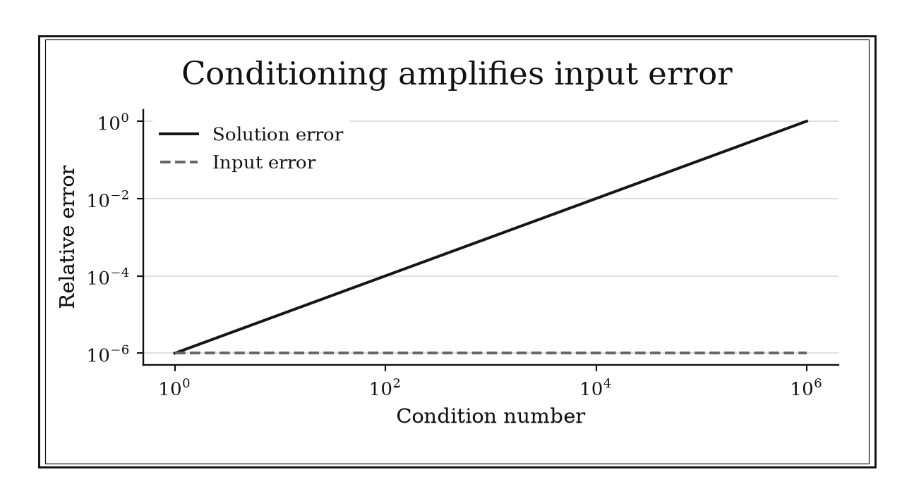
Figure 7.1. For diagonal A=diag(1,1/kappa), perturbing b=(1,0) by (0,10^-6) produces relative solution error kappa times 10^-6. This deliberately aligned example attains the amplification bound.
7.1.2: Check matrix symmetry relative to scale
History
Every numerical-linear-algebra course teaches engineers to test whether a computed matrix counts as symmetric before trusting a symmetry-dependent solver; nobody can point to the paper that proposed comparing against as the decisive test. Attribution chains for this diagnostic lean on the surrounding solver literature, on Cholesky factorization, conjugate gradients, and symmetric eigensolvers, all of which explain why symmetry matters to computation, but none documents a dated event proposing this particular scale-relative ratio. Without a located publication or numerical experiment naming the ratio itself, no origin event clears this book’s evidence bar, leaving an evidence gap. Closing it would need a primary software report or documented failure that names the relative-norm test explicitly. Until such a source surfaces, the fairest description is workflow folklore: a floating-point precaution that spread through software practice long before anyone recorded who first framed it as a ratio.
The equation
For nonzero , measure relative asymmetry by
Roundoff-only asymmetry may be consistent with
where is unit roundoff and reflects assembly depth and error accumulation.
How to read it
A matrix is symmetric when flipping it across its diagonal, swapping entry with , reproduces the same matrix. Computed matrices rarely land on that exactly, so the rule compares the size of the mismatch, , against the size of the whole matrix, , using a norm, a single number summarizing overall magnitude. A ratio near machine roundoff says only a tiny nudge is needed to reach the symmetric average .
That normwise smallness does not certify every entry. A single sizable error sitting in one corner of a large matrix can hide inside an average that still looks tiny, the way one cracked tile can hide in a large floor’s overall smoothness.
Comparing the ratio against assembly and discretization tolerances, rather than machine epsilon alone, is what separates ordinary rounding noise from a genuine modeling or coding error.
How to use it
In a concert hall, an acoustics engineer is building a covariance-like matrix from repeated impulse-response measurements, expecting the reciprocal relationship between source and receiver positions to make it symmetric. Before running a symmetric eigensolver to isolate resonant modes, she computes and , giving
consistent with ordinary rounding across many averaged recordings, and she proceeds with the symmetric solver. On a session where a microphone stand shifted partway through, the same computation instead gives against , so , several orders above her assembly tolerance. Silently averaging with at that point would erase the evidence of the equipment move without correcting it, leaving a falsely tidy matrix that still misrepresents the hall. Instead she traces the discrepancy to the shifted channel and re-measures it before trusting any resonance estimate. This is a Workflow heuristic: it validates a structural precondition before a symmetry-dependent algorithm is allowed to run.
7.1.3: Certify an eigenpair with its residual
History
Trust a solver’s completion flag without question, and a structurally unsound eigenvector can pass straight into a design decision. Turing’s 1948 rounding analysis connected a computed answer to the residual and rounding behavior left behind by the arithmetic that produced it. In modern software terms, that connection means a method’s completion flag is not itself an accuracy certificate. The normalized eigenpair residual here is a modern backward-error diagnostic built on that residual view: it separates the natural scale of the equation from the defect the computed pair still carries.
The equation
For a computed eigenvalue and nonzero eigenvector , let
and report
How to read it
An eigenvector is a direction a matrix does not rotate, only stretches or shrinks, by a factor called its eigenvalue, . Feed a candidate pair back into the matrix and the leftover measures how far it falls short of the exact relationship; dividing by the natural scale of the two terms that should cancel turns that leftover into a dimensionless fraction, , measuring how small a nudge to the matrix would make the pair exact.
For matrices that mirror themselves across the diagonal, a small also pins the true eigenvalue nearby. For a matrix whose directions interact strongly with one another, a tiny can still sit beside a wildly sensitive eigenvalue, so a clean residual does not by itself promise a clean forward answer.
How to use it
A structural engineer computes a candidate vibration mode for a footbridge: eigenvalue estimate and eigenvector normalized to , from a stiffness-and-mass matrix with . The solver reports convergence, but she certifies the pair anyway. The residual is , so
evidence that the pair solves a nearby matrix problem, even though the software offered no accuracy number of its own. A second, closely spaced mode returns a residual at the same scale. Describing the bridge model as mildly nonnormal does not supply a numerical bound on the true frequency error; the engineer still needs a quantitative sensitivity check before signing off. A strongly asymmetric bearing arrangement can make that distinction especially consequential, since a small residual may coexist with a sensitive frequency estimate. This is a Workflow heuristic: it verifies the output of an eigensolver and determines whether refinement or sensitivity analysis must follow.
7.1.4: Equilibrate rows and columns with wildly different scales
History
Should a badly scaled system always be rescaled before it is solved? Practitioners disagree, because what looks like arbitrary numerical noise to one engineer can encode real physical weighting to another. Alan Turing’s 1948 study of matrix computation under finite precision examined how elimination, pivot choices, and rounding interact. Reading that analysis for scale sensitivity, widely separated row and column magnitudes distorting a computation though the equations have not changed, is this book’s modern extension. Turning that reading into a pre-solve step is this book’s answer to the dispute: rescale by default, but only once the disparity has been confirmed as arbitrary rather than meaningful.
The equation
Choose nonsingular diagonal scaling matrices and and solve
The diagonal factors are commonly chosen from row and column magnitudes.
How to read it
Scaling multiplies each row and column of the matrix, the coefficient grid describing the system, by a chosen factor, solves the rescaled system, then undoes the multiplication on the answer. Bringing rows toward comparable size makes pivot choices and leftover-equation checks meaningful; bringing columns toward comparable size makes unknowns recorded in different physical units easier to compare.
Equilibration can improve entry-by-entry behavior and curb harmful growth during elimination. It cannot turn nearly redundant columns into independent ones, and it cannot supply information the original data never had.
For an exact system , nonsingular row scaling preserves the same constraints, while column scaling changes the coordinates of the unknowns. Recover the original solution with ; scales the equations and right-hand side, not the solution vector. In least squares, row scaling instead changes the residual weights and must respect the intended objective.
How to use it
For a field’s nutrient balance, an agronomist models one equation carrying micronutrient coefficients near (parts per million) and another carrying irrigation-volume coefficients near (liters per hectare). Solved without rescaling, the irrigation row can swamp the micronutrient row so completely that the solver effectively ignores the smaller equation. Scaling the micronutrient row by and the irrigation row by brings both toward order one,
and column scaling then lets nitrogen, potassium, and water-volume unknowns be compared on the same footing. Recovering after solving returns the blend recommendation in native units, respecting both constraints instead of quietly satisfying only the large-magnitude one.
For this exact balance system, scaling each entire equation together with its right-hand side leaves every physical constraint unchanged. If the model is changed to a weighted least-squares fit, however, row factors change the objective’s relative weights and must be chosen accordingly. This is a Workflow heuristic: it improves the numerical representation before a solver is applied, but it does not change the exact system’s physical solution or cure intrinsic sensitivity.
7.1.5: Use iterative refinement to recover linear-solve accuracy
History
A factorization computed in reduced precision leaves genuine error in its solution, and refactoring from scratch to fix it wastes most of the original work. The same 1948 analysis singled out residual correction: Turing treated the leftover of an approximate solution as data for another, cheaper solve, alongside his study of conditioning, elimination, and rounding. Modern mixed-precision refinement extends that documented correction process: it computes the residual more accurately than the original factorization allowed and reuses the same approximate factors to correct it.
The equation
Given an approximate solution , repeat
The correction equation may use the same LU or Cholesky factors as the initial solve.
How to read it
The residual, , measures how badly a current candidate answer satisfies the original equations when plugged back in. Solving a new, cheap system for that leftover estimates the error in and adds the estimate back, refining the answer without repeating the expensive part of the work. Evaluating accurately preserves correction information that a lower-precision factorization may already have discarded.
Refinement reuses the same triangular factors each round rather than factoring again; its value comes from those correction solves being far cheaper than the original one.
Successful refinement should shrink both the residual and the correction step together. Once an update stops changing the answer at working precision, further rounds are unlikely to recover anything more.
How to use it
A manufacturing engineer solves a large system of fit equations for a CNC fixture’s compensation offsets using a fast, single-precision LU factorization; the result carries a relative error near , enough to matter at micron tolerances. Computing the residual in double precision and solving with the same factors gives a correction that, added back, contracts the error by roughly the same factor each round, about : after one round, after a second, closing in on double-precision accuracy. The engineer accepts the refined offsets once the scaled residual stops shrinking between rounds rather than after a fixed count of iterations.
On a fixture with a nearly singular clamping geometry, refinement can stagnate early: the correction step stops shrinking well before double-precision accuracy is reached, because the factors are too inaccurate relative to the system’s condition number. Return to the digit budget from Rule 7.1.1 in that case rather than running more refinement rounds hoping they will keep helping. This is a Workflow heuristic: it recovers accuracy and supplies an a posteriori check inside a completed linear-solve process.
7.2: Match the Algorithm to Matrix Structure
Matrix structure is computational information. The nine rules in this section choose factorizations, transformations, storage models, and orderings that preserve accuracy while avoiding work the problem never asked for.
7.2.1: Solve systems instead of forming an explicit inverse
History
Storing a dense inverse costs one million numbers, though a single right-hand side needs only one column’s worth of that information. Turing’s 1948 paper on rounding error studied both routes, solving a system directly and inverting a matrix outright, as part of the same finite-precision analysis of elimination, residuals, and rounding. The modern instruction narrows his broader study to one recommendation: when only the product is wanted, compute it through a solve rather than building every column of the inverse first.
The equation
For a general dense matrix, factor
and solve
When structure permits, use alternatives such as or . In each case, solve without explicitly forming .
How to read it
An inverse, , is the operator that undoes what does to every vector at once; a right-hand side only asks what that operator does to one particular vector. Factoring and running two triangular solves targets exactly that answer. Building the full inverse computes and stores every column the operator could produce, most of which this problem never asked for, then multiplies by anyway.
Choosing between the two routes does not fix a bad matrix: an ill-conditioned stays exactly as sensitive whether solved through factors or through an explicit inverse, and neither route can rescue an answer the problem itself refuses to support accurately.
Factoring costs the most work, paid once. Each further right-hand side needs only two cheap triangular solves, so reuse grows more worthwhile as more arrive.
How to use it
With one fixed interaction matrix, genre-and-title features, a streaming service scores subscriber viewing-history vectors against it. Storage does not decide the route: LU factors and an explicit inverse each need about stored numbers, and flop totals converge too once many subscribers arrive. The real difference is upfront: building the inverse costs roughly three times the factorization alone and is typically less accurate. Factoring once and running two cheap solves per subscriber matches the ranking scores at lower setup cost, without that accuracy penalty.
If the team later needs the diagonal of a covariance-like matrix, say to report how sensitive each genre score is to noisy ratings, inverting the whole matrix for that diagonal still pays the same construction penalty for no benefit; a routine built for diagonal entries specifically skips it. This is a Workflow heuristic: it chooses the computational route for applying an inverse inside a larger problem.
7.2.2: Use partial pivoting for general dense LU
History
A pivot swap skipped in the wrong spot lets a perfectly correct algebraic method return numbers dominated entirely by rounding error. Turing’s 1948 rounding-error analysis examined elimination and pivot choices under finite precision, showing that legal exact-arithmetic steps can behave very differently once tiny pivots meet rounding. Row-pivoted elimination as the standard dense default is modern library practice built on that analysis, adopted to control dangerous division and unchecked growth of intermediate numbers.
The equation
Partial pivoting constructs
choosing at elimination step an entry of largest magnitude among
The permutation matrix records row swaps.
How to read it
Gaussian elimination clears entries below a pivot by dividing lower rows by it and subtracting a multiple of the pivot row. A pivot near zero forces a huge multiplier, which can blow up rounding error and produce enormous intermediate numbers even when the true, exact solution is modest. Swapping a larger entry into the pivot spot before dividing usually keeps those multipliers, and the error they carry, under control.
That word usually matters. Rare matrices still produce large growth even under this swapping rule; it is a strong default, not a guarantee.
The search for a larger pivot looks only within the column currently being eliminated, so the extra safety costs little next to checking every remaining matrix entry.
How to use it
A traffic engineer solves a signal-timing network where one intersection’s flow-balance equation happens to carry a near-zero coefficient, , next to a neighboring equation with coefficient :
Eliminating without a swap divides by that near-zero pivot, creating a multiplier of and a second pivot of similarly enormous magnitude, numbers far outside anything the physical network could produce, so rounding error swamps the true timing solution. Partial pivoting swaps the rows first, uses the pivot , and keeps the multiplier at , small enough that rounding never gets a foothold. The engineer relies on the standard pivoted solver in the signal-optimization software rather than a hand-rolled elimination routine that skips the swap.
Pivoting fixes this particular danger but does not rescue a network whose flow equations are close to genuinely redundant, two intersections whose timings are mathematically forced to move together, say. That kind of near-dependence survives any pivoting choice and needs a separate conditioning check. This is a Workflow heuristic: it selects the stable default factorization path for a general dense system.
7.2.3: Treat Schur complements as first-class operators
History
Applying one generic preconditioner across an entire coupled system can leave the piece that actually controls the remaining unknowns untouched. Issai Schur’s 1917 work in Berlin on matrices and representations included determinant identities now expressed through what is called the Schur complement: eliminating one block of a coupled system algebraically exposes a smaller, reduced operator carrying the eliminated block’s influence on whatever remains. Schur’s is the block identity. Approximating and preconditioning that reduced operator at its own scale is the modern reading: it targets the piece actually controlling what remains.
The equation
Assuming the block is nonsingular, for
eliminating produces the Schur complement
and the reduced equation
How to read it
Split a coupled system into two groups of unknowns, and , with coefficient blocks , , , describing how each group affects itself and the other. Eliminating leaves an equation in alone, governed by : block corrected by the round trip through , an -solve, and . The unknowns that remain see reshaped by everything the eliminated block passed along.
Writing describes what that correction does; a real computation solves with rather than inverting it, and building explicitly can turn a sparse system dense.
can be worse conditioned than either original block, so its difficulty must be measured on its own rather than assumed from .
How to use it
A two-tier distribution network, local depot flows, block , per region, coupled to regional hub throughput, block , , through cross-terms and describing how depot orders draw on hub inventory, is what a logistics planner models. Eliminating the depot-level unknowns leaves a reduced hub system, , governing hub-to-hub transfers alone; formed explicitly it densifies the hub layer to entries, since every hub now interacts with every other hub it shares depots with. Approximating instead from hub throughput volumes keeps the reduced system sparse enough that the solve still finishes overnight.
Assuming the reduced hub system behaves like a simple rescaling of would be a mistake: because folds in the entire depot layer through , it can need a different preconditioner than alone suggests, and the planner checks ’s own scale before sizing that approximation. This is a Workflow heuristic: it reorganizes and preconditions a coupled solve around the operator produced by block elimination.
7.2.4: Prefer QR to normal equations for accurate least squares
History
A matrix’s condition number, squared before solving, doubles the rate at which the problem loses every digit it could have kept. Alston Householder showed in Oak Ridge, Tennessee, in 1958 how elementary unitary transformations, later called reflections, could reduce a matrix to triangular form; his reflections preserve Euclidean length and supply the stable machinery behind QR factorization. Householder gave the norm-preserving triangularization. The payoff is practical: the normal-equation route squares singular values through instead, costing a fit real digits his reflections would have kept.
The equation
For a tall full-rank matrix,
and least squares becomes
The normal-equation route obeys
How to read it
An orthogonal transformation, one that only rotates or reflects without stretching, preserves length exactly; forming instead squares every one of the matrix’s singular values, the stretching factors along its natural axes. The ratio between the largest and smallest of those factors, the condition number, is squared too, and the dot products inside can also lose small information through cancellation.
Normal equations trade some accuracy for a route that can be cheaper to set up. QR represents the same least-squares geometry in an orthonormal basis without first squaring the spectrum.
A tiny diagonal entry surfacing in is a warning to switch to a rank-aware method rather than forcing a full-rank solve.
How to use it
A psychometrician fits a scoring model regressing exam results on twelve item-cluster scores for several thousand students; the design matrix’s condition number is . Solved through normal equations, the effective condition number becomes
Under a small-residual assumption, the rough arithmetic budget suggests about twice as many digits lost through normal equations as through a stable QR route. A substantial least-squares residual can make the original problem itself more sensitive, so alone does not certify the coefficients. The psychometrician uses Householder QR, solves , and checks residual-dependent sensitivity before comparing small coefficients across cohorts.
Had two item clusters been nearly redundant, always tested together, the normal-equation route’s Cholesky step could fail outright, or return coefficients noisy enough to flip sign between cohorts, a rank warning rather than mere inconvenience. QR alone does not repair that redundancy: a suspiciously small diagonal entry in still calls for a pivoted or SVD-based fit. This is a Workflow heuristic: it routes a least-squares problem toward a factorization consistent with its accuracy requirement.
7.2.5: Use Cholesky for symmetric positive-definite systems
History
Assuming a matrix is positive definite because it looks symmetric on paper carries real risk: practitioners disagree how much verification it deserves, and a wrong guess returns a factorization that quietly fails. André-Louis Cholesky developed a square-root factorization around 1910 in French military geodesy, exploiting symmetry and positive definiteness, the property guaranteeing no zero or negative pivot ever appears, to represent a matrix through one triangular factor and its transpose. The factorization is Cholesky’s. The guardrail is modern: it catches the one mistake his shortcut cannot survive, a symmetric-looking input that is not actually positive definite.
The equation
For symmetric positive-definite ,
with positive diagonal entries in . Dense Cholesky requires about
flops, compared with roughly for dense LU.
How to read it
Positive definiteness means for every nonzero vector , ruling out zero or negative pivots during elimination, so no row swaps are needed. Symmetry means only one triangular half of the matrix must be stored and updated. Together the two properties let the matrix be written as , one triangular factor and its own transpose, at roughly half the arithmetic of a general factorization.
The name Cholesky belongs to a factorization needing both properties together; supplying only one does not earn the shortcut.
In floating point, successful positive pivots are good evidence of positive definiteness rather than proof; a tiny pivot needs a scale-aware read, not an automatic pass or fail.
How to use it
From 400 soil-moisture sensors, an environmental scientist builds a spatial covariance matrix to krige contaminant estimates across a watershed; the matrix is genuinely symmetric positive definite once measurement noise is modeled. Cholesky costs about flops against roughly for general LU, and every new sampling date reuses the same factor through two cheap triangular solves.
If duplicated records at identical coordinates are assigned no independent measurement-noise term, the covariance can become singular and Cholesky can fail. An independent positive noise variance preserves positive definiteness even at duplicate coordinates; any added diagonal term should represent an explicit model choice rather than merely hiding a data error. The scientist checks the symmetry ratio and smallest pivots first and only then trusts the factorization. This is a Workflow heuristic: it selects the efficient factorization only after SPD structure has been justified.
7.2.6: Prefer orthogonal transformations for numerical stability
History
Two transformations can be mathematically equivalent and numerically worlds apart. Alston Householder’s 1958 demonstration that elementary reflections could triangularize a matrix while preserving Euclidean length reaches past the least-squares case already covered here: any orthogonal or unitary map shares that same length-preserving property. Preferring such transformations as the default building block whenever an equivalent choice exists is the broad modern workflow drawn from his result.
The equation
For an orthogonal matrix ,
so
For complex matrices, replace transpose by conjugate transpose and “orthogonal” by “unitary.”
How to read it
An orthogonal matrix, , satisfies : multiplying by it only rotates or reflects a vector, never stretching or shrinking it, so for every , and its condition number is exactly , the best possible. Undoing the transformation costs nothing extra either, since .
That safety belongs to the transformation itself. An orthogonal step cannot make an already ill-conditioned problem worse, but it also cannot fix the conditioning that problem already had.
Because preserves inner products, angles and orthogonality between vectors survive the transformation too, which is why these maps recur across least squares and eigenvalue work.
How to use it
A photogrammetry engineer aligns drone-camera frames using rotation matrices computed from matched ground-control points. Rather than building each rotation from raw trigonometric products that can drift from true orthogonality after repeated composition, the pipeline represents each update as a Givens rotation or Householder reflection, guaranteeing by construction: a ground point at relative position meters maps to under the calibrated rotation, since , the same distance preserved exactly. Composing such frame-to-frame rotations along a flight path preserves every ground-point distance the same way.
After many finite-precision compositions, the accumulated rotation can drift slightly away from true orthogonality even though each individual step was orthogonal by construction; the engineer periodically re-orthogonalizes the running product rather than assuming the guarantee holds forever, and never lets the composed rotation silently absorb a lens-distortion error it was never meant to correct. This is a Workflow heuristic: it chooses stable transformations inside factorizations, least-squares solvers, and eigenvalue algorithms.
7.2.7: Go matrix-free when storage dominates arithmetic
History
Eighty gigabytes: that is what a dense matrix costs to store in double precision, more than most machines have. Cornelius Lanczos published a short-recurrence eigenvalue iteration while working in Los Angeles in 1950, building a Krylov subspace, information from repeated matrix-vector products, without forming a full factorization. Lanczos’s iteration is historical; exposing only the matrix’s action on a vector, never its stored entries, is the modern large-scale consequence of that structure.
The equation
A dense binary64 matrix requires approximately
When can be computed from a stencil, transform, or Jacobian-vector product, matrix-free storage is often
for state and work vectors.
How to read it
A Krylov method learns about a matrix only through what it does to vectors, repeated products , and inner products built from them, never through individually stored entries. Skipping assembly saves memory and the traffic of moving a huge matrix through the machine.
Being matrix-free does not remove the need for a preconditioner; access to alone can still leave an iteration too slow to finish.
When both and are supplied, testing on random vectors can catch an inconsistent implementation before an iterative method absorbs the error.
How to use it
Across a -node regional aquifer grid, a hydrologist models groundwater flow. Storing the full coefficient matrix densely would need
beyond the workstation’s memory, but each node’s equation only involves its immediate neighbors, so a stencil routine computes directly from the grid, and working vectors fit in a few hundred megabytes.
Before trusting a new stencil implementation, she checks it against a small assembled matrix on a coarse grid and verifies the adjoint relation numerically, since a boundary-condition bug in matrix-free code fails silently: the wrong answer looks plausible, and only a dense check would have caught it. This is a Workflow heuristic: it changes representation and solver architecture when matrix storage, rather than arithmetic, is the binding constraint.
7.2.8: Use blocked matrix algorithms to exploit fast BLAS-3 kernels
History
Two routines can perform the exact same number of arithmetic operations and finish hours apart. Around 1990, the LAPACK project reorganized dense linear-algebra software, work carried out across the United States and United Kingdom, so that most computation could be expressed through Level 3 BLAS matrix-matrix kernels, reusing data already sitting in fast memory. That blocked design is documented in LAPACK’s own working notes; the block sizes that work best remain hardware-dependent tuning choices the project never fixed once and for all.
The equation
Choose a block size so active panels and tiles use fast memory effectively, then group trailing updates into operations such as
This GEMM-like update performs many arithmetic operations for each fetched block of data.
How to read it
Moving data through the memory hierarchy is often slower than operating on it. A matrix-matrix kernel, one large operation like , reuses each loaded block of numbers many times over, while single-column updates stream the same large matrix past the processor again and again for comparable arithmetic.
Blocking changes data movement far more than it changes the algebra, which is why a library routine can outrun a mathematically identical hand-written loop by a wide margin.
The rule says blocking helps; it does not say which block size to pick, an architecture-dependent tuning choice. Below some problem size, blocking’s own overhead exceeds the reuse benefit, and an unblocked routine wins.
How to use it
A manufacturing engineer runs an overnight finite-element crash simulation whose dominant cost is a sequence of dense triangular factorizations on blocks. Written as single-column updates, the routine streams each trailing block past the processor once per column, about passes; reorganized to update columns at a time as matrix-matrix products, the same arithmetic runs as roughly passes, each a highly reused block operation. Switching to the vendor-BLAS-backed LAPACK routine cuts the overnight run from nine hours to under two, from data reuse alone.
Running that routine on a batch of small sub-assembly checks shows no such speedup and can even run slower, since call overhead and copying small arrays now dominate whatever a matrix-matrix kernel could reuse. This is a Workflow heuristic: it selects an implementation organization that preserves the mathematics while matching modern memory hierarchies.
7.2.9: Reorder sparse factorizations to control fill
History
A sparse matrix with only a handful of nonzeros per row can still exhaust a machine’s memory once elimination runs, because a poor ordering turns zeros into new nonzeros far faster than expected. Alan George analyzed nested dissection, recursively splitting a problem’s connectivity graph into separated pieces, for sparse positive-definite grid systems while working in Stanford, California, in 1973; his recursive separators confine much of the new nonzero structure elimination creates. The historical algorithm directly targets fill. Choosing a permutation before factorization begins is the modern first-pass workflow built from it.
The equation
For an SPD factorization or general LU, write
The decisive memory measure is often
not merely .
How to read it
Eliminating one unknown connects all of its remaining graph neighbors to each other, the way removing a load-bearing wall forces adjacent rooms to share a new beam; those new connections are called fill, and a sparse matrix can end up nearly dense after enough eliminations. A permutation, an order in which unknowns are eliminated, does not change the underlying equations but can change how much fill appears.
A good ordering removes low-connection unknowns early and saves the most connected ones, the separators, for last, limiting how large any one clique of new connections grows.
A chosen ordering does not guarantee numerical stability: pivoting can override it for an indefinite or badly scaled matrix, so actual fill can depart from the symbolic estimate.
How to use it
For a building’s finite-element mesh, degrees of freedom with about seven nonzeros per row, nonzeros total, a structural engineer factors the stiffness matrix. Factored in the mesh’s natural node numbering, a bad ordering lets elimination fronts grow so wide the factor needs on the order of GB, well under the GB a fully dense triangular factor would need ( doubles, bytes). Reordering with nested dissection, splitting the mesh recursively along its natural separators, confines most fill near those separators, and the factorization completes in about GB, a tenfold reduction.
The engineer records the factor nonzero count and peak memory rather than trusting input sparsity or the ordering algorithm’s promise alone. This is a Workflow heuristic: it reduces the storage and work of a sparse direct solve before numeric elimination begins.
7.3: Estimate Spectra, Compression, and Iterative Difficulty
Spectral information predicts both opportunity and cost. The nine rules in this section screen eigenvalues, forecast iteration rates, price low-rank compression, define usable rank, and escalate specialized Krylov tactics only when the evidence warrants them.
7.3.1: Use Gershgorin disks as a cheap eigenvalue screen
History
A skipped plausibility check on a computed eigenvalue lets a coding error return a spectrum nobody would believe if they looked. Semyon Gershgorin published a theorem while working in Leningrad in 1931 placing every eigenvalue of a matrix inside a union of disks built only from diagonal entries and off-diagonal row sums. The disk theorem is his; using it as a cheap plausibility screen before trusting a full eigensolver is the modern operational choice built on it.
The equation
For row , define
Then every eigenvalue lies in
Each disk is centered at with radius .
How to read it
For each row, add the absolute values of every off-diagonal entry to get a radius, , and center a disk on that row’s diagonal entry. Every eigenvalue of the matrix must fall inside the union of all those disks; the theorem needs nothing but a scan of the matrix’s own numbers.
The bound is cheap because it is loose: heavily overlapping disks can cover most of the plane and rule out very little.
If every disk sits strictly in one half of the plane, so does every eigenvalue, and a computed value outside that region is immediately suspect.
How to use it
A sports-analytics team builds a rating-adjustment matrix from head-to-head results across a twelve-team league. Two illustrative rows give disks centered at radius , spanning to , and at radius , spanning to . Scanning all twelve rows’ diagonal-dominance margins, the analyst confirms every disk lies right of , so an eigenvalue near is impossible; when a bug returns exactly that value, she rejects it on sight.
A disk-cleared eigenvalue still needs its own check: disks overlapping heavily elsewhere would leave the true eigenvalue anywhere across their shared region, so clearing the screen is not itself evidence of accuracy. This is an Independent rule: row data directly supplies a guaranteed spectral enclosure without computing an eigenvalue.
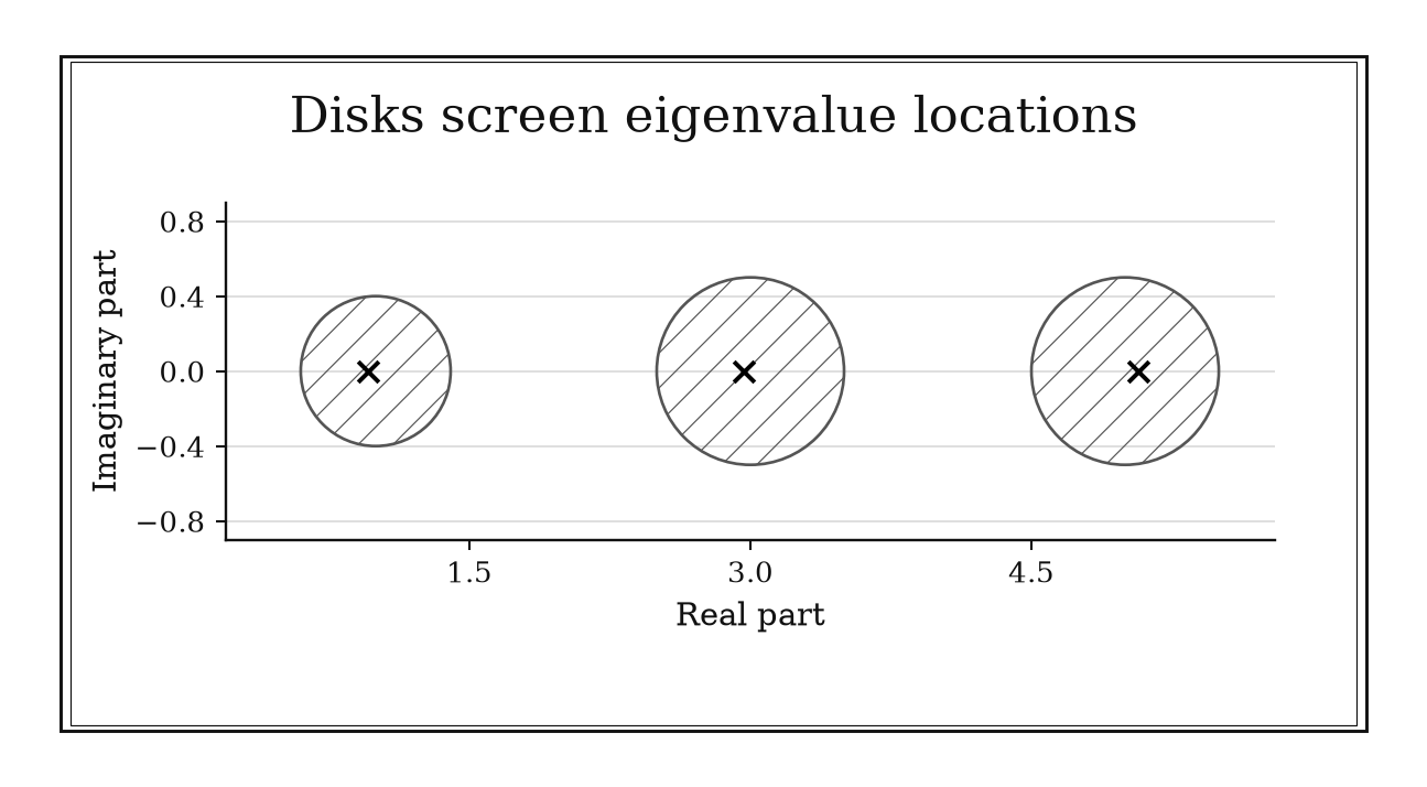
Figure 7.2. The eigenvalues of the displayed construction fall inside the union of its row-based Gershgorin disks. A disk need not contain exactly one eigenvalue; the theorem concerns the union.
7.3.2: Power iteration speed is set by the eigenvalue ratio
History
Repeatedly multiplying by a matrix looks like a toy method to some and a genuinely useful one to others; the disagreement turns on a ratio most practitioners never check first. Cornelius Lanczos’s 1950 Krylov iteration extracted spectral information from repeated matrix-vector products; plain power iteration is the simpler mechanism underneath that result, the same repeated multiplication without Lanczos’s added recurrence. The ratio rule here is the modern first-pass forecast for how fast that simpler mechanism actually converges.
The equation
Normalize repeated products:
If is diagonalizable, its eigenvalues are ordered so that , and the starting vector contains the dominant component, then
How to read it
Write a starting vector as a mix of the matrix’s natural directions, its eigenvectors; each multiplication scales the component along direction by that direction’s eigenvalue, . Normalizing after each step removes the common growth from the dominant direction, , leaving every unwanted direction shrinking relative to it at rate . The nearer that ratio sits to one, the slower the unwanted directions fade.
This forecast concerns direction only; the eigenvalue estimate itself and its residual need a separate check.
A negative dominant eigenvalue can make the normalized vector flip sign every step while still converging to the same one-dimensional line.
How to use it
Refreshed nightly by repeated multiplication, the dominant eigenvector of a co-purchase matrix ranks items for a recommendation engine. With , ten passes shrink the unwanted component by about , plenty for a stable nightly ranking. During a flash sale, two items briefly draw nearly identical purchase volume, pushing the ratio to ; reaching that same separation would now take roughly passes, far more than the nightly batch window allows, so the top-item ordering keeps flickering between the two.
The engineering team switches to a Lanczos-based method for that window rather than running plain power iteration longer, since a ratio this close to one is exactly the regime the simpler iteration handles poorly. This is an Independent rule: the eigenvalue ratio directly forecasts dominant-mode iteration speed under its stated spectral assumptions.
7.3.3: Use shift-invert for interior or smallest eigenvalues
History
Ordinary power iteration finds only the largest eigenvalue; it cannot home in on one sitting in the middle of the spectrum. In 1950, Lanczos showed the same repeated matrix-vector action could build a subspace rich enough to extract spectral information without factoring the matrix. Shift-invert targeting reuses that machinery on a transformed operator: shift the spectrum so the interior eigenvalue of interest becomes the extremal one, and ordinary Krylov iteration finds it directly.
The equation
If
then for a shift ,
Eigenvalues nearest become largest in transformed magnitude.
How to read it
Pick a shift, , a number near the eigenvalue actually wanted, and apply Krylov iteration to instead of itself. Every eigenvalue becomes under this transform, so whichever eigenvalue sits closest to turns into the largest transformed value, exactly what power-style iteration is good at finding.
That gain costs one linear solve per iteration instead of one plain multiplication; the transformed problem is only as trustworthy as those shifted solves.
One factorization of can often be reused across every iteration, so setup cost is paid once.
How to use it
A recording-studio acoustician wants the control room’s resonant mode nearest a vocalist’s lowest sustained note, not the room’s loudest overall mode. With eigenvalues at , , and in normalized frequency units and a shift , the transformed values become
so the mode at dominates the transformed problem and a short Krylov run isolates it directly.
Moving the shift closer to an actual mode, to for example, makes more sensitive to perturbations and can reduce solve accuracy; the acoustician checks the residual back in the original problem rather than trusting the transformed eigenvalue’s apparent dominance. This is a Specialized heuristic: it escalates to an expensive spectral transformation when ordinary extremal methods cannot reach the desired part of the spectrum.
7.3.4: Check low-rank storage before compressing a matrix
History
A dense table of one million numbers is the artifact this rule interrogates before anyone compresses it: does a proposed low-rank replacement actually take less room? Carl Eckart and Gale Young published a theorem in Chicago in 1936 characterizing the best possible approximation of a matrix by one of lower rank; in modern language, keeping a matrix’s leading singular components, its strongest independent directions, gives the optimal low-rank approximation for the relevant norm. Eckart and Young proved the optimality; counting factor entries first is newer bookkeeping, catching a rank too costly to store.
The equation
An dense matrix stores
numbers. Rank- factors and store approximately
Storage savings require
How to read it
A dense table stores numbers, one for every row-column pairing. A rank- replacement stores two much smaller tables instead, roughly numbers total, whose product reconstructs an approximation of the original. The break-even point, , is pure bookkeeping: it marks when the replacement is smaller, a separate question from whether it approximates the original well.
For a square table, that threshold sits near half the table’s side length, far less restrictive than the rank a useful approximation usually needs.
Multiplying by the compressed factors also costs roughly operations instead of , so a genuinely low-rank replacement can save arithmetic as well as storage.
How to use it
A table of survey responses, respondents against question-and-brand pairs, sits with a market-research firm that wants to know whether a rank- summary is even worth building before checking its accuracy. Dense storage needs numbers; a rank- factorization needs , a twentyfold reduction, comfortably under the break-even point .
That count says nothing about whether rank actually captures real structure in the responses; a firm that stops here and skips the singular-value check risks shipping a compressed table that saves storage while discarding a meaningful cluster of dissenting respondents the raw entries still held. This is an Independent rule: it directly decides whether a proposed factor rank can save raw storage before compression begins.
7.3.5: Use the next singular value to price a low-rank approximation
History
Compressing an image to a handful of components without checking what gets discarded hides exactly how much was given up, information the very next singular value would have revealed. Carl Eckart and Gale Young’s 1936 theorem on optimal low-rank approximation supplies that certificate: no other matrix of the same rank can do better in the relevant norm. Their result is the optimality guarantee; spending the discarded singular values as a budget, not discovering the loss by accident, is the newer habit.
The equation
For the rank- truncated SVD,
the errors are
How to read it
A matrix’s singular values, , rank how strongly it stretches space along each of its natural, mutually independent directions. Truncating to rank leaves a worst-case error, in the spectral norm, of exactly , the very next value discarded; adding the squares of every value past gives the squared Frobenius error instead.
A steep drop after makes compression attractive; a slowly fading tail means each extra rank buys little.
The theorem promises optimal error in these norms only. Sparsity is separate: the compressed matrix usually loses it when error looks small, and the guarantee is silent on signs and which entries a decision needs.
How to use it
An imaging team compresses a satellite photo whose only nonzero singular values are , , , and ; keeping rank leaves a worst-direction error of and a Frobenius error of
Moving to rank instead drops both errors to , a tenfold improvement for one extra component, so the team accepts the modest storage cost of rank over rank for this image.
A small measured error in either norm does not guarantee the compressed photo preserves what an analyst actually needs, a faint vehicle-sized feature or a sharp shoreline edge, since the SVD’s optimality is blind to any single feature that does not carry much overall signal energy; the team validates the rank- result against those specific features before archiving the original at full resolution. This is an Independent rule: the singular-value tail directly prices the best achievable rank- matrix error.
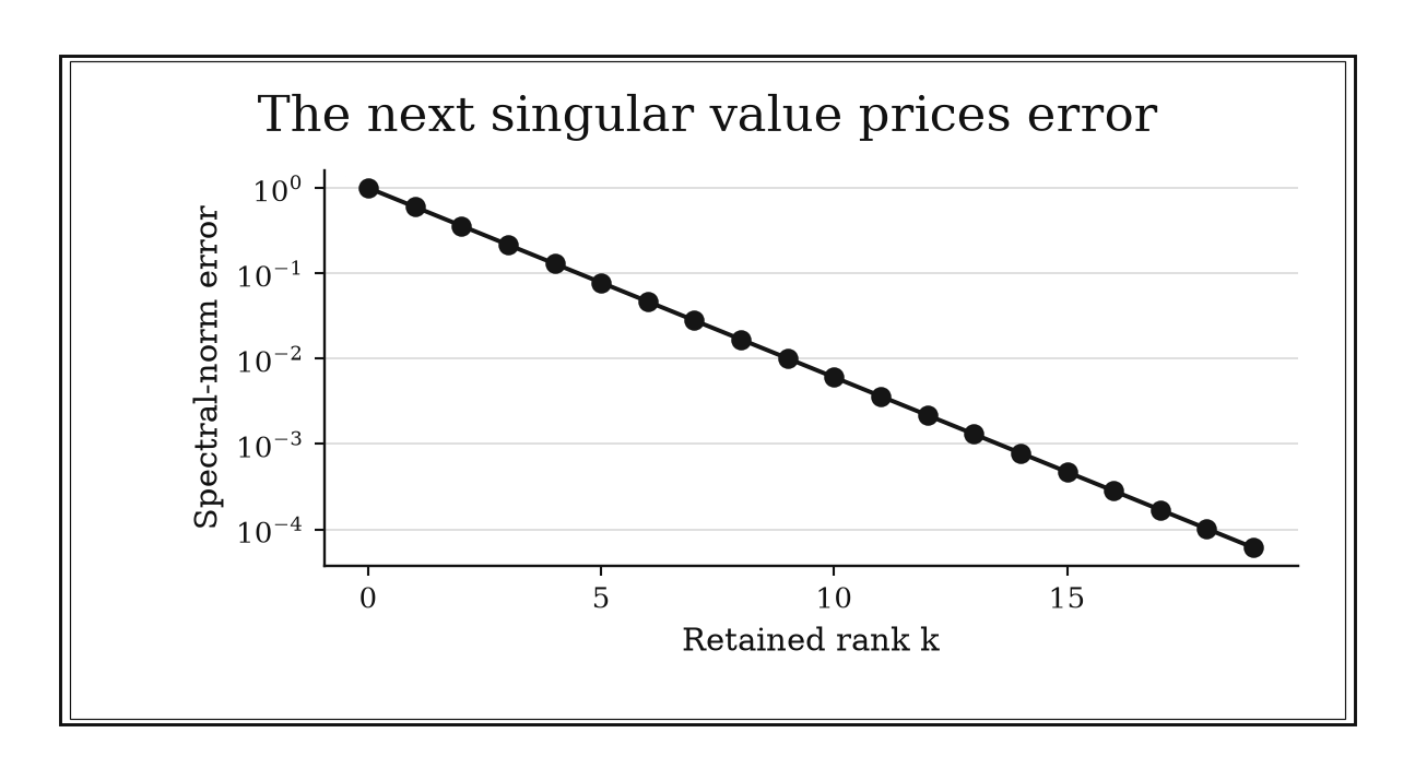
Figure 7.3. For a constructed diagonal matrix with singular values 0.6^(j-1), the best rank-k spectral-norm error equals sigma_(k+1). This is a norm-specific statement, not an entrywise guarantee.
7.3.6: Define numerical rank relative to the largest singular value
History
A computed singular value tested for exact equality to zero almost never triggers the test, since rounding rarely lands exactly on it. Gene Golub and William Kahan published stable bidiagonalization-based machinery for computing singular values and the pseudoinverse while working in Stanford, California, in 1965, helping turn the singular value decomposition into a dependable numerical instrument. Golub and Kahan’s contribution was the stable computation. Defining rank against scale, arithmetic, and data noise, rather than exact zero, is the modern habit that keeps their computation trustworthy.
The equation
For singular values
define numerical rank by
A roundoff baseline is
for an matrix, where is the machine-precision constant used by the routine. A common binary64 convention takes ; conventions that call half this value “unit roundoff” differ only by a factor of two.
How to read it
Singular values measure how strongly a matrix stretches space along each of its independent directions; the largest, , sets the natural scale for the rest. Numerical rank counts how many singular values clear a threshold built from that scale and the arithmetic’s roundoff level, rather than counting how many are exactly nonzero, a test computed data essentially never satisfies cleanly.
The roundoff-based threshold reflects only the arithmetic; measurement noise in the data can be far larger and should set the threshold instead.
Rank can jump abruptly as crosses a tight cluster of singular values, so a stable count across plausible thresholds is stronger evidence than one default number.
How to use it
Fields against measured properties fill a matrix of soil-sensor readings that an agronomist has on hand. With , the roundoff baseline is
but a spectral-norm bound on the sensor-noise matrix is , almost eight orders above the arithmetic floor, so the agronomist sets and counts only singular values clearing that physical threshold.
Using the roundoff baseline instead would count singular values the sensors cannot actually distinguish from noise, inflating the apparent number of independent soil factors. This is a Workflow heuristic: it converts singular values into a defensible usable-rank decision tied to precision and data quality.
7.3.7: Expect conjugate-gradient work to scale with square-root conditioning
History
Leave a system badly conditioned, and a solver that should finish in ten steps can grind through a thousand instead. Magnus Hestenes and Eduard Stiefel introduced the conjugate-gradient method for symmetric positive-definite systems in 1952, working between Los Angeles and Zurich; later analysis connected its practical iteration count to how spread out or clustered the matrix’s eigenvalues are. The method and its convergence structure belong to Hestenes and Stiefel. The square-root planning rate is a modern shortcut: it lets an engineer budget passes before running a single iteration.
The equation
In exact arithmetic, for SPD , CG error satisfies the worst-case bound
where
How to read it
Conjugate gradient searches for the best approximate answer within an expanding space built from repeated multiplications, judged by an energy measure, . That search behaves like a polynomial that must stay small across the matrix’s eigenvalues, from to ; squeezing that range, , into a narrower one lets a lower-degree polynomial do the job, which is where the rough iteration count comes from.
The bound is a worst case: eigenvalues clustered into a few tight groups can converge far faster than the raw ratio predicts.
The residual monitored during a run is cheap, but the bound is stated in the energy norm of the true error, a different, unobservable quantity.
How to use it
A utility engineer solves a linearized power-flow system for a regional grid, symmetric positive definite after the standard reference-bus reduction, with condition number . Plain conjugate gradient needs on the order of iterations per fixed digit of accuracy; a diagonal preconditioner tuned to the grid’s admittance structure drops to , and the iteration scale falls to , a hundredfold reduction in solver passes.
Before reusing that preconditioner on next month’s grid topology, the engineer confirms it stays symmetric positive definite under the new configuration; a topology change breaking that property would make plain CG invalid outright, converged-looking residuals notwithstanding. This is an Independent rule: conditioning supplies a transferable first estimate of CG difficulty before a large solve is attempted.
7.3.8: Judge a preconditioner by clustered eigenvalues and total time
History
Does the preconditioner that cuts iteration count the most always win? Not if each of those iterations costs enough more to erase the savings. Hestenes and Stiefel’s 1952 conjugate-gradient method made spectral structure the thing to manage, its conjugate directions and later polynomial analysis explaining why a clustered, well-scaled spectrum converges faster than a spread-out one. Judging a preconditioner by total time, not iteration count, is the modern refinement between looking good on paper and finishing faster.
The equation
Apply through approximate solves and work with
For SPD and , the ideal trend is
with eigenvalues clustered away from zero.
How to read it
A preconditioner, , is a cheap stand-in for whose approximate solves reshape the system’s effective spectrum before each conjugate-gradient step. The ideal result clusters the transformed eigenvalues tightly and pulls them away from zero, since a low-degree polynomial suppresses error fastest over a tight cluster.
Applying means solving through the preconditioner representation rather than constructing a dense inverse, and that cost belongs in the timing budget. Ordinary preconditioned CG requires the applied action to remain a fixed symmetric positive-definite linear map. Variable or nonlinear approximate inner solves need a compatible flexible method and its own convergence checks.
A useful total-cost model is setup time plus iterations times per-iteration cost; the preconditioner with the fewest iterations does not automatically minimize that sum.
How to use it
Via conjugate gradient, a manufacturing engineer runs a thermal simulation of a furnace’s steady-state temperature field. Unpreconditioned, the solve takes iterations at ms each, s total. An algebraic multigrid preconditioner takes ms to build and cuts the run to iterations at ms each:
a clear win despite each iteration costing eight times as much. A second candidate preconditioner halves the iteration count to but triples the per-iteration cost to ms:
slower overall than doing nothing at all, even though it looks like an improvement by iteration count alone.
The engineer adopts the multigrid preconditioner and keeps timing both iteration count and wall-clock cost on future furnace geometries, since a preconditioner tuned for one mesh can lose its clustering advantage, and its time advantage with it, once the geometry changes enough. This is a Workflow heuristic: it evaluates and tunes a solver component by spectral effect and end-to-end cost together.
7.3.9: Increase GMRES restart when convergence stalls
History
Restarting an iterative solver saves memory, but it can also discard useful search directions, leaving the iteration barely progressing. Yousef Saad and Martin Schultz introduced GMRES for nonsymmetric systems in New Haven, Connecticut, in 1986: a method minimizing the residual over an expanding space of matrix-vector products, at a storage cost their paper confronts directly. Saad and Schultz own the method and its storage tradeoff. Raising the restart length once convergence stalls is the specialized response, trading memory for a run that finishes.
The equation
For a restart cycle of length in dimension , basis memory scales roughly as
while orthogonalization work over a cycle scales roughly as
Restarting discards the old Krylov basis and begins again from the current residual.
How to read it
A restart cycle of length keeps only the last search directions before restarting from the current residual, at a memory cost near and an orthogonalization cost near . Full GMRES, with no restart, keeps searching a continuously growing space and never discards a direction.
A short restart can repeat nearly the same weak cycle, since whatever the previous cycle failed to suppress is what the next cycle starts from again.
Watching the true residual’s reduction factor at each restart boundary separates ordinary stalling from trouble caused by scaling or finite precision instead.
How to use it
A logistics planner solves a nonsymmetric flow-balance system for a one-way trucking network, using restarted GMRES with at . Storing those vectors costs bytes, GB, but convergence stalls: the true residual barely shrinks between cycles.
Raising the restart to needs bytes, GB, and the same run converges in one cycle instead; cycle-boundary residuals before the change show the same weak factor repeating, evidence the short restart was discarding directions the network’s asymmetric costs needed. Pushing far higher would make orthogonalization, scaling with , expensive enough to erase the gain. This is a Specialized heuristic: it adjusts a nonsymmetric Krylov method only after restart-induced information loss is visible in the convergence history.
Chapter Synthesis: Diagnose, Match, and Verify
Reliable matrix computation begins before the first factorization. Conditioning limits how much accuracy is available. Relative structural checks decide whether symmetry-dependent methods are legal. Residuals certify what a solver actually achieved, equilibration improves the numerical representation, and iterative refinement can recover information left in a correctable equation defect.
Algorithm choice should then follow matrix structure. Solve for the action of an inverse rather than constructing it. Use pivoted LU for a general dense system, Cholesky for verified SPD structure, and QR when least-squares accuracy matters. Treat block elimination, orthogonal transformations, matrix-free actions, cache blocking, and sparse ordering as mathematical-computational choices rather than afterthoughts.
Finally, let the spectrum price difficulty. Gershgorin disks provide a cheap enclosure; eigenvalue ratios forecast power iteration; shift-invert targets otherwise inaccessible modes. Storage counts and singular-value tails decide whether low rank is worthwhile, while tolerance defines numerical rank. Conditioning and clustering predict Krylov work, and restart length mediates GMRES memory against retained information.
Across all twenty-three rules, ask four questions:
- What accuracy can the problem permit before algorithmic error is considered?
- Which structural property has been verified rather than assumed?
- What storage, data movement, or fill cost accompanies the arithmetic?
- Does the rule answer the problem, guide the workflow, or justify a specialized escalation?
One-Page Linear Algebra Toolkit
| Recognition cue | Rule to try | What it gives | Role |
|---|---|---|---|
| Condition estimate and precision budget | Subtract from available digits | Attainable-accuracy estimate | Independent |
| Matrix claimed symmetric | Compute | Structural gate | Workflow |
| Computed eigenpair | Scale by | Backward-error certificate | Workflow |
| Rows or columns span many orders of magnitude | Equilibrate diagonally | Better numerical representation | Workflow |
| Factorized solve has residual accuracy left | Apply iterative refinement | Accuracy recovery | Workflow |
| Need | Factor and solve | Direct action without full inverse | Workflow |
| General dense system | Use row-pivoted LU | Stable default factorization | Workflow |
| Coupled block system | Expose the Schur complement | Reduced operator and preconditioner target | Workflow |
| Accurate dense least squares | Use Householder QR | Avoid squared conditioning | Workflow |
| Verified SPD system | Use Cholesky | Half-cost symmetric factorization | Workflow |
| Choice of equivalent transformations | Prefer orthogonal or unitary operations | Norm preservation | Workflow |
| Operator action cheap, storage unaffordable | Go matrix-free | -scale storage path | Workflow |
| Dense arithmetic is memory-bound | Use blocked BLAS-3 algorithms | Data reuse and throughput | Workflow |
| Sparse direct factorization | Reorder before elimination | Lower fill and peak memory | Workflow |
| Need a fast spectral enclosure | Build Gershgorin disks | Guaranteed eigenvalue screen | Independent |
| Dominant eigenpair iteration | Inspect | Convergence forecast | Independent |
| Interior eigenvalue target | Apply shift-invert | Transformed extremal problem | Specialized |
| Proposed low-rank factorization | Compare with | Storage break-even | Independent |
| Truncated SVD | Inspect and tail energy | Best-possible error price | Independent |
| Rank decision in noisy arithmetic | Declare a scale-aware | Numerical rank | Workflow |
| Large SPD Krylov solve | Estimate work from | CG difficulty scale | Independent |
| Candidate preconditioner | Compare spectrum and total time | End-to-end solver value | Workflow |
| Restarted GMRES stagnates | Test a larger restart | Memory–convergence tradeoff | Specialized |
Decision Path
- Start with sensitivity. Estimate conditioning and the digit budget before setting solver tolerances.
- Verify claimed structure. Check relative symmetry, positive definiteness, sparsity pattern, block meaning, and scale before choosing a specialized factorization.
- Choose the direct method by matrix type. Use Cholesky for verified SPD systems, pivoted LU for general dense systems, and QR or SVD for least squares according to conditioning and rank.
- Avoid unnecessary objects. Solve for inverse actions, apply Schur complements through block solves, and keep orthogonal factors implicit when possible.
- Budget memory as well as flops. Consider matrix-free actions, cache blocking, and fill-reducing ordering before the matrix outgrows the machine.
- Verify outputs. Scale residuals, inspect orthogonality where relevant, and refine a solve only while backward error continues to improve.
- For spectra and compression, inspect cheap evidence first. Use Gershgorin, eigenvalue ratios, storage counts, and singular-value tails before escalating to shift-invert or large decompositions.
- For Krylov methods, separate problem difficulty from solver design. Check SPD requirements, conditioning, clustering, preconditioner cost, restart behavior, and true residuals.
Transfer Problems
1. Build an accuracy and method budget
A binary64 least-squares matrix has and is reported to have full column rank. Under a small-residual assumption, estimate the rough arithmetic digit budget for QR and for normal equations. Explain why a substantial residual would require a fuller conditioning analysis, and state what residual, rank, and scaling checks you would require before accepting either result.
2. Route one matrix through the workflow
A sparse matrix is advertised as symmetric positive definite, but and its rows span twelve orders of magnitude. Decide what to inspect and scale before choosing Cholesky or CG, and explain why simply replacing by is not yet justified.
3. Price spectral information
A matrix has singular values . Compare dense storage with a rank- factorization, state its spectral-norm error, and explain how a spectral-norm data-noise bound of changes the numerical-rank decision. Then name the extra evidence needed before trusting that compression in a downstream application.
Where These Ideas Reappear
- Analysis: operator norms and condition numbers become quantitative stability constants, while residuals become backward-error certificates.
- Optimization: Hessian structure selects Cholesky, KKT systems create Schur complements, and preconditioning controls Krylov subproblems.
- Numerical methods: pivoting, refinement, orthogonal transformations, and tolerance-aware rank are central stability mechanisms.
- Scientific computing: blocking, matrix-free operators, sparse ordering, and total-time accounting connect algorithms to hardware.
- Differential equations and PDEs: discretizations generate sparse SPD, saddle-point, and matrix-free systems whose structure determines the solver.
- Statistics and data science: least squares, covariance matrices, SVD truncation, and numerical rank control regression and compression.
- Control and signal processing: eigenvalue location, conditioning, low-rank models, and interior modes determine stability and reduced-order behavior.
Historical Notes and Sources
The historical profiles distinguish documented algorithms and theorems from modern tolerances, implementation thresholds, and workflow language. The relative-symmetry profile remains an explicit evidence gap.
- Turing on conditioning, elimination, residuals, and rounding: Turing’s 1948 paper and the King’s College Cambridge archive record.
- Schur and block elimination: MacTutor biography of Issai Schur.
- Householder and orthogonal triangularization: scan of Householder’s 1958 paper and the ACM record.
- Cholesky and geodetic systems: Numdam historical study reproducing Cholesky’s manuscript and MacTutor biography of Cholesky.
- Lanczos and matrix-vector eigenvalue iteration: NIST scan of Lanczos’s 1950 paper and the NIST Krylov-method history page.
- LAPACK’s blocked design: LAPACK Working Note 24 and the Netlib LAPACK history and FAQ.
- George and sparse nested dissection: DOI record for George’s 1973 paper and the SIAM nested-dissection paper.
- Gershgorin’s eigenvalue disks: MacTutor biography of Semyon Gershgorin.
- Eckart and Young on low-rank approximation: original Psychometrika paper and SIAM historical notes on the SVD.
- Golub and Kahan on practical SVD computation: original SIAM paper and SIAM historical notes on SVD computation.
- Hestenes and Stiefel on conjugate gradients: NIST scan of the 1952 paper and the NIST conjugate-gradient history page.
- Saad and Schultz on GMRES: original GMRES paper and Netlib Templates for the Solution of Linear Systems.
- Evidence-gap and modern numerical practice: LAPACK Users’ Guide and Higham, Accuracy and Stability of Numerical Algorithms. These support the mathematics and surrounding need, not an exact origin event for the relative symmetry test.