Chapter 8: Number Theory: Reduce Large Arithmetic to Small Structure
A number can be too large to write down and still be easy to reason about. The final digit of an enormous power may depend on a cycle only four steps long. Two large integers may surrender their greatest common divisor after a few remainder operations. A question about hundreds of possible factors may collapse into independent choices among a handful of prime exponents.
Number theory repeatedly rewards the same move: preserve the structure that matters while discarding the size that does not. Remainders preserve divisibility information. Prime factorizations turn multiplication into exponent bookkeeping. Coprime moduli let one problem split into smaller ones and then reassemble without ambiguity.
The ten rules in this chapter form three families. The first extracts divisibility information without unnecessary enumeration. The second makes modular arithmetic a controlled process of reduction and reconstruction. The third distinguishes tasks that look similar but demand different methods: testing one small candidate, listing many primes, shortening a huge exponent, or tracking the depth of one prime factor.
The governing question is: what smaller representation preserves exactly the integer property the problem asks about?
8.1: Extract Divisibility Information Efficiently
Factoring is powerful, but it is not the universal first move. A greatest common divisor can be found without factoring either input. A divisor count becomes immediate once a factorization is known. A prime count at a large scale may need only a density estimate. The efficient method depends on the requested output.
8.1.1: Use remainders instead of factoring to find a gcd
History
Must a common divisor of two large numbers be found by factoring both and comparing, or is there a route that skips factoring? Book VII’s opening propositions in Euclid’s Elements described such a route: repeatedly remove the smaller number from the larger until the common measure becomes visible. Modern division compresses those subtractions into one step, writing and continuing with and . The notation changed; the payoff, an exact gcd without factoring, did not.
The equation
For integers and with ,
For the computation, start from and and repeatedly take nonnegative remainders until one is zero. The last nonzero value is the nonnegative gcd.
How to read it
Dividing by leaves a quotient (how many times fits) and a remainder , so . The quotient can be discarded: any integer dividing both and also divides , and any integer dividing and also divides . The two pairs share exactly the same common divisors; only the pair keeps shrinking, the way 252 and 105 shrink to 105 and 42 in a few steps. It answers only the gcd question, not either number’s prime factors.
How to use it
A machine shop needs the tooth ratio between a 252-tooth gear and a 105-tooth gear reduced to its simplest whole-number form before cutting new blanks. The foreman skips factoring and reduces by remainders:
The gcd is 21, so the ratio reduces to , and the shop orders a 12-tooth and a 5-tooth blank instead of two odd sizes. Reversed, those same equations also supply the forward pass for the modular-inverse method in Rule 8.2.2.
The shortcut assumes both counts are exact; from only a measured center distance and an approximate ratio, the gcd it returns can mislead. Do not factor first unless the prime factors are themselves wanted. This is an Independent rule: it produces a gcd directly across arithmetic, algebra, cryptography, and rational computation.
8.1.2: Read the divisor count from prime exponents
History
Listing every divisor of a large number by hand risks missing one, with no easy way to confirm the count is complete. With Disquisitiones Arithmeticae in 1801, Gauss brought divisibility, residues, congruences, and prime-power structure under one system. That viewpoint made it natural to replace a list of divisors with the choices that generate it: once a number is decomposed into prime powers, which integers divide it becomes which exponent is chosen for each prime.
The equation
If
where the are distinct primes and , then the number of positive divisors is
How to read it
A positive divisor of has the form , with for each prime factor. Prime offers possible exponents, 0 through , and since choices for distinct primes never interact, they multiply the way shirt colors multiply by sizes to give a count of outfits. Add one to each exponent, then multiply: that is the whole formula. It counts how many divisors exist without constructing them; it does not say what they are.
How to use it
A library-stacks supervisor has 360 identical boxes to shelve and wants to know how many rectangular layouts, so many boxes per row times so many rows, are possible before comparing them for aisle width. Factoring first,
each divisor pairs a row count with a column count: 2 to the 0th through 3rd power (4 choices), 3 to the 0th through 2nd (3 choices), 5 to the 0th or 1st (2 choices). Therefore
Because 360 is not a perfect square, twenty-four divisors form twelve complementary row-and-column pairs, and a 20-by-18 layout is the same cart as an 18-by-20 layout turned sideways, so the supervisor screens twelve layouts, not twenty-four.
The count only holds if 360 already reflects every box; if a few are pulled for damage first, the supervisor must refactor the new total rather than subtract from 24. This is an Independent rule: after factorization is available, it directly answers divisor-count questions in many settings.
8.1.3: Estimate prime counts by n over log n
History
On the Number of Primes Less Than a Given Magnitude, an 1859 memoir of a few pages, took the known approximation to the prime count and asked why it works. Bernhard Riemann began from the known approximation to the count of primes below a bound and recast the problem through the complex zeta function, whose explicit formula explained corrections to the rough density scale . That first-order density survives on its own as a useful estimate: not a prediction of the next prime, but a scale for how many primes a large interval likely contains.
The equation
Let denote the number of primes at most . The prime number theorem states
meaning
where is the natural logarithm.
How to read it
Near a large scale , the rough density of primes is about (natural logarithm, a slowly growing number: about 14 at a million, 21 at a billion). Roughly one integer out of every near size is prime, thinning out only gradually as grows. This is an asymptotic statement about relative error: the wavy symbol says the ratio of the true count to this estimate approaches one, even though their absolute gap can keep growing. It gives a scale, not a location.
How to use it
A systems engineer is scoping a project needing a table of every prime below one million, useful for choosing hash-table sizes, and wants the job’s scale before writing the exact sieve. At , , so
against the true count . The estimate misses by thousands, low, but correctly prices the table’s size: tens of thousands of entries, enough to plan memory before the exact count is in hand.
The formula cannot say whether one candidate size is itself prime, and it says nothing about how primes are spaced within the interval; it only justifies the budget, not the search itself. This is an Independent rule: it gives a portable scale estimate wherever the aggregate abundance of primes matters.
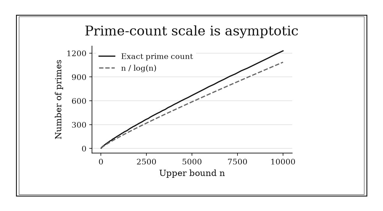
Figure 8.1. Exact sieve counts and n/log(n) show the same broad growth. The approximation is visibly low over this finite range; asymptotic equivalence is not a finite error certificate.
8.2: Solve Congruences by Reducing and Reconstructing
A congruence records only a remainder class, so carrying full integers through every intermediate line wastes information the question will discard. Reduce early, determine when division is legal, and split a difficult modulus when coprime pieces make the arithmetic easier.
8.2.1: Reduce modulo m at every arithmetic step
History
An intermediate number carried far past what the final question needs costs memory and time once fixed-size arithmetic enters the picture. In 1801, Gauss’s Disquisitiones Arithmeticae organized number theory around congruence notation, divisibility, residues, and unique factor structure. Writing turned “has the same remainder” into a relation that could be manipulated systematically; large representatives no longer had to dominate the page. Reducing at every step is the payoff of that shift: any convenient representative may stand in throughout addition and multiplication.
The equation
If
then
and
How to read it
Congruent integers modulo (the modulus, the number you take remainders against) differ by a multiple of , the way 37 and 7 differ by a multiple of 10. Adding, subtracting, or multiplying them changes an expression only by another multiple of , so the final residue survives; you may choose small residues or a balanced one like instead of . Division is different: canceling from is valid only when shares no factor with ; skip that check and the cancellation can be wrong.
How to use it
A credit union clerk is auditing a legacy batch system that tags each account record with a check digit equal to the last digit of and needs to confirm one flagged tag by hand. Rather than expanding , the clerk reduces at every step:
The check digit should read 1; the batch system shows 3, so the clerk sends the record back for reprocessing.
The method only certifies the digit the modulus protects: reducing modulo 10 destroys nearly everything else the account number carried, so this check catches a corrupted tagged digit, not a transposition elsewhere. This is a Workflow rule: it keeps every line of a larger modular calculation small and valid.
8.2.2: Use extended Euclid to find modular inverses
History
Ordinary division by a nonzero number is defined; division modulo can fail outright, since modular arithmetic has no built-in reciprocal. Euclid’s gcd procedure, set out in the Elements, supplied the forward reduction steps needed to repair that failure long before anyone phrased it in terms of inverses. Substituting those equations backward produces coefficients expressing the gcd as a combination of the two original numbers, and when that gcd is one, the same coefficients manufacture the modular reciprocal division alone could not.
The equation
Bézout’s identity gives integers and such that
Therefore has an inverse modulo exactly when . In that case,
so is an inverse of modulo .
How to read it
That identity names and as whatever integers make equal the gcd of and , a pair guaranteed to exist for any and . Reduce the equation modulo and the term vanishes, leaving , precisely what it means for to be ’s inverse. If the gcd is , this can never happen, since every combination of and is divisible by , and 1 is not. The same calculation also solves : solutions exist exactly when the gcd of and divides . The inverse is the number that undoes multiplication by 7 on a 26-hour clock: 15 steps of 7 make four full turns and land one position past the start.
How to use it
A cryptography engineer is building the decryption side of a simple affine cipher over the 26-letter alphabet and needs the inverse of encryption multiplier 7 modulo 26. Euclid’s steps run forward,
then reverse,
So , and ; a check confirms it, .
The construction only works because ; a multiplier sharing a factor with 26, such as 4, would leave no inverse to find, and the cipher would map multiple letters to one ciphertext letter, a flaw to catch before deployment. This is an Independent rule: it both decides invertibility and constructs the inverse for modular equations, reconstruction, and cryptographic arithmetic.
8.2.3: Split coprime congruences with the Chinese remainder theorem
History
Know a number’s remainder against several small, unrelated moduli, and you can reconstruct the number itself, up to one large repeating range, without ever seeing it directly. The Sunzi suanjing, compiled in China between the third and fifth centuries, posed a now-famous version of this puzzle: find a number leaving specified remainders when divided by , , and . Its constructive solution is an early documented instance of the structure now called the Chinese remainder theorem.
The equation
For pairwise coprime moduli , the system
has exactly one solution modulo
With and , one construction is
How to read it
Each product in the reconstruction acts like a selector: congruent to 1 modulo its own and 0 modulo every other modulus, the way a light switch controls only its own circuit. Multiplying it by installs the desired residue in one channel without disturbing the others, and summing the selectors combines every requirement at once. Coprimality, the moduli sharing no common factor, guarantees the needed inverses exist and makes the answer repeat only after the full product of the moduli.
How to use it
A facilities scheduler runs two recurring maintenance routes, a 3-day route currently due in 2 days and a 5-day route due in 3 days, and wants the next day both land on together. Modulo 15, the selector for the 3-day route is 10, reading 1 modulo 3 and 0 modulo 5, and the selector for the 5-day route is 6. Therefore
Counting 8 days out, both routes coincide, and every 15 days after, since 3 and 5 share no common factor.
If a third route on a 6-day cycle is folded in, the theorem stops applying directly, since 6 shares a factor with 3, and the period is no longer the plain product of all three numbers. This is an Independent rule: it directly reconstructs an answer and also transfers across scheduling, coding, parallel arithmetic, and modular algorithms.
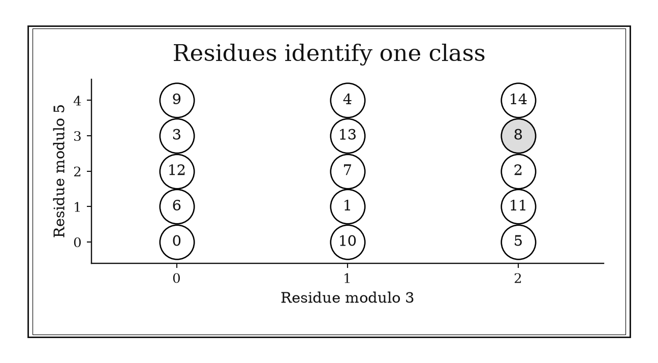
Figure 8.2. The residues modulo three and five pair each integer from 0 through 14 with a different grid cell. The pair (2,3) identifies 8 modulo 15 because the moduli are coprime.
8.3: Match Prime and Power Structure to the Task
“Work with primes” is not a complete algorithm choice. One small candidate calls for bounded trial division. Every prime below a limit calls for a sieve. A huge power modulo a number calls for periodicity. A divisibility question about one chosen prime calls for a valuation. Match the representation to the workload.
8.3.1: Test divisors only through the square root
History
Attribution chains for the square-root stopping rule reach for the sieve of Eratosthenes, the one genuinely documented practice nearby, but that sieve answers a different workload: producing many primes together, not testing one candidate, so its story clears none of this book’s evidence bar. A hand primality check needs to run only through the square root, an argument any reader can verify without historical evidence at all, but nobody can point to the moment that stopping rule became doctrine, leaving an evidence gap. Closing it would need a primary text stating the square-root stopping point for a single candidate, with a defensible date. Until then, the fairest account is folk mathematics.
The equation
If is composite and
then
Consequently, if no prime divides , then is prime.
How to read it
Factors of a composite come in pairs sitting on opposite sides of (the square root, the number that multiplied by itself gives ): if both and exceeded , their product would overshoot . So a composite is guaranteed a factor at or below its square root, and checking that far proves primality with certainty. Only prime candidates need testing: if is not divisible by 2, there is no need to test 4 or 6 either. The method leaves open how long the check takes once , and so , grows very large.
How to use it
A city clerk certifying a small special-election petition has exactly 97 valid signatures and needs to know, before assigning review teams, whether that count splits into equal-sized groups at all. Because
only the primes below 10, 2, 3, 5, and 7, need checking. The number is odd, its digit sum is not divisible by 3, it does not end in 0 or 5, and , so none divides it. Ninety-seven is prime, confirmed with four checks rather than ninety-six.
The method is fast here only because 97 is small; a countywide count in the millions would make checking every prime up to its square root far too slow by hand. For one huge number use a suitable primality test; for all primes through a bound use Rule 8.3.2. This is a Workflow rule: it sets a rigorous stopping point inside a single-number factor or primality search.
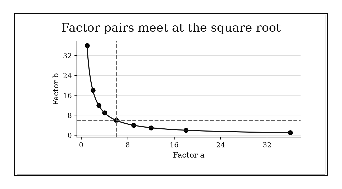
Figure 8.3. For n=36, every factor pair has a member at or below six. The square pair meets the boundary exactly; trial division must include a divisor equal to the square root.
8.3.2: Use a sieve when you need many primes at once
History
Should every integer in a range prove its own primality independently, or can one confirmed prime do work on behalf of many candidates at once? The sieve attributed to Eratosthenes, who worked in Alexandria in the third century BCE, answers with the second option: list the integers and repeatedly strike out multiples, so one discovered prime eliminates an entire arithmetic progression of composites in a single pass. The modern rule of thumb reframes that as a workload decision: invest once in a prime table when many later questions can reuse it.
The equation
To sieve through , when a prime is reached, mark
Begin at because smaller multiples of already have a smaller prime factor. No new sieving prime is needed after
How to read it
Every composite up to a limit has a prime factor no bigger than , the pairing idea behind the square-root primality test, so crossing out multiples of every prime up to removes every composite in range; whatever survives above 1 is prime. Crossing out multiples of can safely start at , since any smaller multiple of was already crossed out by a smaller prime. The advantage is doing the work once: one pass answers many later prime-or-not questions, though the table itself costs memory proportional to how far it reaches.
How to use it
A math teacher planning a semester of worksheets, most asking students to spot primes below 30, builds one reusable table instead of re-testing each candidate by hand every time. Listing 2 through 30, mark 2’s multiples starting at 4, then 3’s still-unmarked multiples starting at 9, then 5’s starting at 25; since the next prime, 7, exceeds , no further sieving prime is needed. The survivors are
ten primes the teacher prints on every worksheet and quiz for the rest of the term.
The table pays for itself only once reused; for a single homework question, sieving to 30 would cost more than testing that number directly. A full sieve uses memory proportional to the bound, so a table into the thousands is built in segments. This is a Workflow rule: it selects a collective prime-generation method when repeated queries can share the preprocessing cost.
8.3.3: Reduce modular exponents using the group period
History
A modular exponent with hundreds of digits cannot simply be expanded and then reduced: the intermediate number would dwarf any computer’s memory before a single remainder could be taken. Between 1736 and 1741, Leonhard Euler, working in St Petersburg and Berlin, published proofs of Fermat’s assertion about powers modulo a prime and developed its broader totient-based generalization. The result exposed a periodicity beneath such calculations: powers of an invertible base eventually repeat, so once the base is verified invertible, its exponent can be replaced by a much smaller one and reduced by its period.
The equation
For a prime not dividing , Fermat’s little theorem gives
More generally, if , Euler’s theorem gives
where counts the invertible residue classes modulo .
How to read it
The invertible residues modulo form a finite multiplicative group: multiply any two and the result stays inside it, so repeated powers of an invertible element must eventually cycle back to the start. Euler’s totient , the count of numbers from 1 to sharing no factor with , is a guaranteed group-wide cycle length, so raising an invertible base to that many steps, or any multiple, returns 1. Exponents differing by a multiple of give the identical residue; that guaranteed period need not be the smallest one for a particular base.
How to use it
A cryptography engineer needs to verify a signature check requiring modulo the small prime 7, standing in for a much larger real modulus. Since 7 is prime and does not divide 3,
Since ,
Nearly the entire exponent, small here but scaling the same way, disappears before any large integer forms.
The shortcut fires only because 3 and 7 share no common factor; applied to a base sharing a factor with the modulus, the periodicity guarantee would not hold, and the reduced exponent would give a wrong answer with no warning. Composite moduli may be easier after factorization and Chinese-remainder reconstruction. This is a Workflow rule: it transforms one stage of a modular-power calculation after its structural conditions have been checked.
8.3.4: Use p-adic valuations to track prime-power divisibility
History
A number system built around a single question, how deeply does one chosen prime divide this quantity, is what Kurt Hensel introduced in 1897, working in Marburg. His p-adic numbers measured arithmetic by powers of a chosen prime, where divisibility by a high power of counts as closeness rather than smallness in the ordinary sense. The valuation used here is the bookkeeping core of that viewpoint: record only how many times one chosen prime divides a number, letting every other prime factor drop out of the ledger.
The equation
For a prime and a nonzero integer , define by
Set so the sum rule also covers exact cancellation. For nonzero and ,
and
with equality in the second relation when the two valuations differ.
How to read it
, the -valuation of , is a count: how many times prime divides into before it stops dividing evenly. Multiplication adds prime exponents, so . For a sum, factor out the smaller common power of ; at least that much divisibility survives, more if both terms share the same valuation and their remaining parts cancel modulo . Valuation tracks depth, not size: and differ by only one though a million dwarfs ninety-six.
How to use it
A distribution center receives a combined shipment of units, 40 cartons packed 12 to a case, and the floor manager needs to know how many times that count halves exactly before an odd leftover forces an uneven batch, without multiplying the sizes out first. Because
multiplying batch sizes adds those counts,
The combined 480 units halve cleanly five times, into 240, 120, 60, 30, and 15, before 15 refuses to split evenly.
Had the manager instead added the two batches rather than multiplied them, the shortcut weakens: , matching only the smaller count, not their sum. This is a Workflow rule: it serves as a prime-specific ledger inside divisibility proofs, factorial calculations, gcd work, and cancellation checks.
Chapter Synthesis: Preserve the Property, Shrink the Representation
Number theory becomes manageable when large magnitude is separated from relevant structure. A remainder replaces an integer while preserving its congruence class. The Euclidean algorithm replaces a pair with a smaller pair while preserving every common divisor. A prime factorization replaces a divisor list with independent exponent choices. A valuation throws away every prime except the one whose depth matters.
Method choice still comes first. Use when only the scale of a prime population is needed; it cannot certify any individual prime. Use bounded trial division for one small candidate and a sieve for a reusable interval. Use exponent periodicity only after checking coprimality. Use the Chinese remainder theorem when coprime components are easier than the combined modulus.
Across all ten rules, ask four questions:
- Which property must the shorter representation preserve?
- Does the task concern one integer, many integers, or an asymptotic population?
- Which coprimality, factorization, or size condition makes the shortcut valid?
- Does the rule deliver the answer, or does it organize one stage of a longer calculation?
One-Page Number Theory Toolkit
| Recognition cue | Rule to try | What it gives | Role |
|---|---|---|---|
| Two integers share unknown factors | Repeatedly take remainders | Exact gcd | Independent |
| A full prime factorization is known | Add one to each exponent and multiply | Number of positive divisors | Independent |
| Only the scale of the prime population matters | Use | First-order prime-count estimate | Independent |
| Modular intermediates are growing | Reduce after every addition or multiplication | Smaller equivalent computation | Workflow |
| Modular division is needed | Run extended Euclid | Invertibility test and inverse | Independent |
| Several coprime remainder conditions are given | Apply the Chinese remainder theorem | Unique combined residue | Independent |
| One modest integer may be prime | Test primes only through | Rigorous stopping boundary | Workflow |
| Many primes or repeated queries are needed | Build a sieve | Reusable prime table | Workflow |
| A modular exponent is enormous | Verify coprimality and reduce by a period | Small equivalent exponent | Workflow |
| Only one prime’s divisibility depth matters | Track | Additive exponent ledger | Workflow |
Decision Path
- Do you need a gcd but not a factorization? Use the Euclidean algorithm. Record its equations if an inverse or Bézout coefficients may be needed next.
- Is a complete factorization already known? Translate exponent choices directly into a divisor count. Do not enumerate divisors unless the list itself is required.
- Do you need an aggregate prime estimate? Use for scale. If you need exact primes, choose between trial division, a sieve, and a larger-scale primality method based on workload.
- Is the answer requested modulo ? Reduce throughout addition and multiplication. Before dividing, test invertibility with a gcd.
- Can the modulus be separated into coprime factors? Solve the smaller congruences and reconstruct with the Chinese remainder theorem.
- Is the obstacle a huge exponent? Verify coprimality, identify a valid group period, and reduce the exponent before powering.
- Is the question about the power of one prime in a product, sum, factorial, or gcd? Replace full integers with valuations and watch for equal-valuation cancellation.
Transfer Problems
1. From gcd to legal modular division
Use the Euclidean algorithm to find . Decide whether has an inverse modulo . Then explain, without guessing an inverse, what the gcd tells you about the number of solutions to
2. Split, shorten, and reconstruct
Find modulo if
Reduce each exponent using a justified period, then combine the two residues with the Chinese remainder theorem. State where coprimality is used in each stage.
3. Choose the prime workflow
For each task, choose the first rule you would use and justify the workload choice: test whether is prime; produce every prime below for repeated queries; estimate how many primes lie below ; and determine the highest power of dividing . Do not use one prime method for all four tasks.
Where These Ideas Reappear
- Algebra: Euclid extends to polynomials, while quotient rings generalize modular arithmetic.
- Combinatorics: the divisor-count formula is a product-rule argument over exponent choices.
- Graph theory and algorithms: sieving illustrates amortized work, preprocessing, and time-memory tradeoffs.
- Cryptography: modular inverses, fast exponentiation, coprimality, prime generation, and Chinese-remainder reconstruction are core operations.
- Computer arithmetic: reduction controls overflow and lets large calculations run through fixed-size representatives.
- Coding theory: finite fields and residue structures support error-detecting and error-correcting codes.
- Complex analysis: prime counting connects to the zeta function, turning an integer-distribution problem into an analytic one.
- Local and algebraic methods: valuations isolate one prime at a time and organize lifting, divisibility, and local-global reasoning.
Historical Notes and Sources
The profiles distinguish documented events from modern operational readings. The square-root trial-division profile remains an explicit evidence gap; the historically verified sieve story is not used as a substitute for a different algorithm.
- Euclid and the gcd algorithm: Clark University edition of Euclid, Book VII; Clark University table of contents for the Elements.
- Gauss, congruences, and prime-factor structure: Library of Congress digitization of Disquisitiones Arithmeticae; Smithsonian Libraries digitization.
- Riemann and prime counting: Trinity College Dublin edition and translation of Riemann’s 1859 paper; Clay Mathematics Institute overview.
- The Sunzi remainder problem: National Diet Library of Japan history of the Chinese remainder theorem; MacTutor context for Sun Zi.
- The sieve of Eratosthenes: MacTutor biography of Eratosthenes.
- Euler and modular exponent periodicity: Euler Archive record for work on Fermat’s theorem; MacTutor biography of Leonhard Euler.
- Hensel and -adic arithmetic: EuDML record and scan of Hensel’s 1897 paper; scholarly history of Hensel and -adic numbers.
- Modern number-theory methods and conventions: Victor Shoup, A Computational Introduction to Number Theory and Algebra; MIT OpenCourseWare, Mathematics for Computer Science.