Chapter 9: Combinatorics: Counting Without Exhaustion
Thirteen people enter a room. Without asking anyone’s birthday, we already know that two share a birth month. There are only twelve month categories, so placing thirteen people among them forces a collision. No pair was listed, and no calendar was consulted.
That tiny argument captures combinatorics at its most useful. Counting is often presented as enumeration: write down every case and hope none is missed or repeated. Strong counting begins earlier. Are the alternatives disjoint? Does order matter? Are objects identical or labeled? Is the unwanted case easier to count? Does symmetry identify several descriptions of the same object? Can a recurrence remember only the boundary information needed for the next step?
The eighteen rules in this chapter form three families. The first produces counts and guarantees directly. The second organizes a counting workflow before formulas are chosen. The third recognizes scale and recurring patterns, middle binomial coefficients, logarithmic search depth, derangements, entropy, generating functions, and Catalan structures. Together they support one governing habit: count the structure, not the cases.
A correct formula applied to the wrong notion of “distinct” is still a wrong count. Define the objects, choices, and equivalences before arithmetic begins.
9.1: Counts That Stand on Their Own
Some counting structures are complete enough to answer the question immediately. These six rules turn overcrowding, binary membership, identical objects, sparse selections, overlap, and uniform symmetry into direct counts or guarantees.
9.1.1: Use the ceiling form of pigeonhole
History
A ruler marked into equal short intervals is the entire apparatus behind one of number theory’s cleanest arguments. Working in Berlin in 1842, Dirichlet was chasing rational approximations to a real number: he dropped the fractional parts of many multiples of that number onto the ruler’s intervals. With more fractional parts than intervals, some interval had to catch two of them, and their difference produced the approximation he wanted. The principle predates him; this is the documented use that carried his name into the textbooks. What the crowding bought him was existence without search: the two points never had to be found, only guaranteed.
The equation
If objects are assigned to boxes, where is a positive integer, then
where is the occupancy of box .
How to read it
is the count of objects, the count of boxes, and how many objects land in box . Average occupancy is , but no box holds a fractional object: 25 objects in 4 boxes average 6.25. Rounding that average up, the ceiling, forces some real box to be at least that crowded, like ten coats on eight hooks forcing one hook to carry two; if every box held one less, all boxes together could not hold objects. The rule proves some box is overloaded. It does not say which one.
How to use it
A lab technician must pack 100 sealed sample tubes into 12 storage boxes. Since , at least one box must hold nine or more tubes, so boxes that hold only eight cannot suffice. To show that capacity nine is enough, the technician explicitly balances the load: four boxes receive nine tubes each and eight boxes receive eight, for tubes.
The ceiling proves only a lower bound on the busiest box; the balanced assignment supplies the matching upper bound. If a tube were mistakenly logged in two boxes at once, the partition itself would be invalid until the record is corrected. This is an Independent rule: a valid partition and two integers directly produce a transferable occupancy guarantee.
9.1.2: Remember that an n-set has two to the n subsets
History
Reciting Sanskrit verse correctly depended on knowing every valid rhythm a line could take, since a missed pattern meant a lost meter. Pingala’s Chandaḥśāstra and later commentaries built procedures for listing metrical patterns of long and short syllables, using recursive binary methods and, for a line of given length, powers of two; dates and attribution are disputed. The prosodists counted metrical patterns, not modern subsets; choosing which syllable positions count as “long” is the modern set-theoretic reading over that doubling. A catalog of meters is trustworthy only once every choice at every position has been counted, exactly what doubling guarantees.
The equation
For a finite set with ,
where includes both the empty set and itself. Equivalently,
How to read it
is a finite collection and the list of all its subsets, empty set and whole set included. Each of the members of is either in a given subset or out of it, two states per member, so the tally of subsets is multiplied by itself times. A phone with 12 optional settings has possible on/off combinations, over four thousand, because every extra switch doubles the catalog already available. The rule counts every subset once each. It says nothing about which subsets meet some further condition, such as containing exactly three members; that narrower question needs a different count.
How to use it
A caterer offering a build-your-own sandwich station has 12 optional toppings and wants to know how many distinct sandwiches the counter can produce, since the fridge only holds enough prepped ingredients for a fixed range of combinations. Every topping is independently on or off, so the catalog size is , plain to fully loaded. Confirming the fridge can restock fast enough, the caterer prices the station as unlimited customization.
A regular then asks for a special limited to exactly three toppings. That changes the question: the count is not but , since fixing how many toppings must be chosen removes the independent choice at every other topping. Quoting 4096 for that special would overstate the options badly. This is an Independent rule: unrestricted membership choices directly determine the complete subset count in any finite setting.
9.1.3: Use stars and bars for identical items in labeled boxes
History
Light quanta treated like tiny labeled balls gave physicists a radiation formula that did not match experiment. In 1924, working between Dhaka and Berlin, Satyendra Nath Bose set that assumption aside and rederived Planck’s radiation law by counting how indistinguishable light quanta occupy energy states, without asking which quantum is which. Einstein translated the paper, arranged its publication, and extended the same statistics to material particles. Bose’s full argument layers in degeneracies beyond this book’s scope, but the counting shift he made is the reusable step below: identical items in labeled containers earn a different formula once identities stop mattering.
The equation
For integers and , the number of nonnegative integer solutions of
is
How to read it
Picture identical stars in a row, standing for the items, with bars slotted among them marking off boxes: stars before the first bar belong to box 1, stars between two bars to the next box, and so on; two bars side by side just mean an empty box. Every arrangement of stars and bars names one split of the items, so counting arrangements counts splits: choose which of the positions hold bars, giving . The count assumes boxes are distinguishable and can hold any number of items, including zero. It says nothing about a maximum capacity per box; that restriction needs a separate calculation.
How to use it
A small parts manufacturer has 8 identical fasteners left on the line at shift’s end and must log how they could be split among 3 labeled bins feeding tomorrow’s three stations, since inventory won’t close out the shift until every legal split is accounted for. Solving
the count is
possible splits, including ones where a bin sits empty overnight.
Supervisors dislike an empty bin, since it means a missed changeover, so they ask how many splits keep every bin stocked instead. Writing reduces the problem to , giving splits with every bin holding at least one fastener. Quoting the unrestricted count of 45 to satisfy that requirement would overstate the options, since more than half of those 45 leave some bin bare. This is an Independent rule: identical items, labeled unlimited boxes, and a total directly determine the count.
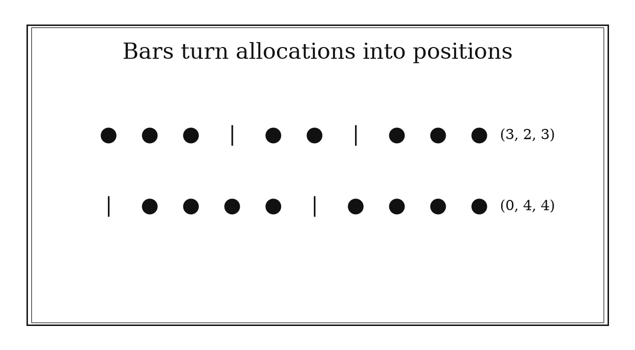
Figure 9.1. Eight identical items and two separators encode allocations among three labeled bins. Adjacent separators allow an empty bin. Choosing the two separator positions among ten gives 45 allocations.
9.1.4: Approximate choose n k by n to the k over k factorial
History
Replace the exact falling product inside a binomial coefficient with a plain power of , and for small the substitution costs almost nothing, a shortcut Siméon Denis Poisson leaned on in 1837 while working in Paris on binomial trials with many opportunities and rare successes. Approximating by was one algebraic step inside his derivation of the limiting law that now bears his name, not a standalone rule he named on its own. The shortcut below isolates that one step so it can be reused wherever a small number of successes is drawn from a much larger pool.
The equation
For integers , exactly,
When is small,
The ratio of the exact count to the approximation is
How to read it
is the pool size, the small number chosen, and the exact product . When stays small next to , each factor sits close to itself, so replacing every factor by plain gives , an estimate that runs high because every substituted factor was rounded up. How high depends on , not just : the accumulated shortfall behaves like
the sum of the small relative losses . The estimate is an asymptotic scale, not a guaranteed error bound of any particular size; enough small losses can still add up to a noticeable one.
How to use it
An auditor sampling a company’s 1000-entry transaction ledger needs a fast estimate of how many distinct 3-entry samples exist, to judge whether a sampling plan avoids predictable coverage gaps. The exact count is
while the shortcut
is close enough for planning. Their ratio,
shows the estimate running about high, matching the correction scale above. Satisfied the two agree this closely, the auditor signs off on the faster estimate for the planning memo rather than computing the exact figure by hand.
The same shortcut would mislead if the sample size grew toward the middle of the ledger’s population; there, Rule 9.3.4’s entropy scale describes the count, not this falling-product estimate. This is an Independent rule: after checking , it directly estimates a broad family of sparse-selection counts.
9.1.5: Subtract overlap after adding two sets
History
Adding the deals in which position one matches to the deals in which position two matches overshoots the true number of matching deals, a discrepancy Pierre Rémond de Montmort had to resolve between 1708 and 1713 in Paris while analyzing the card game Treize, where plain addition overcounted since matches at both positions were tallied twice. Resolving it meant subtracting the overlap back out, the first of an alternating sequence of corrections. Modern set notation postdates Montmort; the correction he needed is the two-set identity below.
The equation
For finite sets and ,
The same equation holds for finite measures or probabilities when cardinalities are replaced consistently.
How to read it
and are two possibly overlapping collections, and is what they share. Adding and counts every shared element twice, once from each collection, so subtracting removes one of those extra copies and leaves every element counted once. For three collections, subtracting every pairwise overlap removes a triple-overlap element too many times, so the next correction adds it back; the pattern keeps alternating as more collections join. Explicitly,
The rule assumes and are drawn from the same universe with a shared, consistent notion of membership; comparing counts built on different conventions breaks the subtraction.
How to use it
A city permitting office wants to know how many active licenses need a health inspection or a fire inspection, since inspectors are budgeting next quarter’s visits. Records show 50 licenses flagged for health, 33 for fire, and 16 for both, since those businesses serve food over open flames. Adding and correcting,
67 licenses need at least one inspection, and the office schedules exactly that many visits rather than the 83 a naive sum would suggest.
A quick check keeps the number honest: , here , and it does. If a third category joined, such as noise complaints, subtracting all three pairwise overlaps would remove any triply flagged license one time too many; the office would need to add that overlap back before trusting the total. This is an Independent rule: two set sizes and their overlap directly determine the union count across many applications.
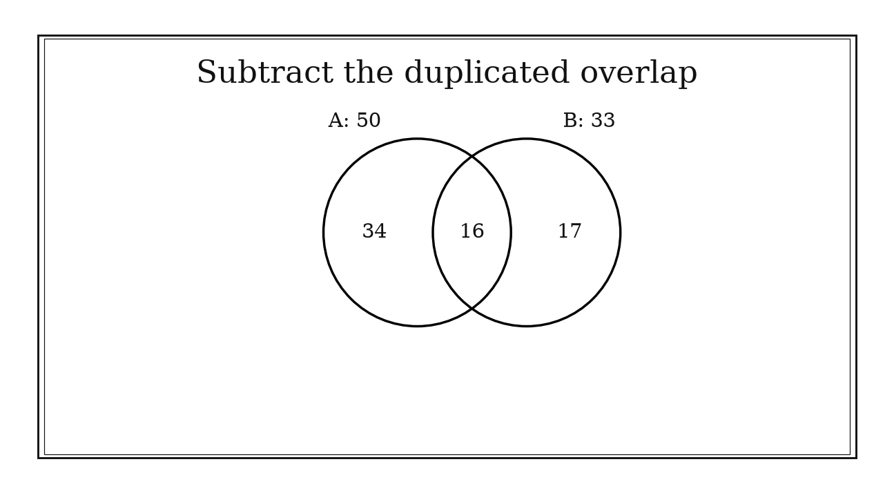
Figure 9.2. Counts 50 and 33 with overlap 16 give a union of 67. The labeled regions are counts; circle areas are schematic and are not proportional to those counts.
9.1.6: Divide by symmetry only when every orbit has the same size
History
How many truly different ways can six people be seated around a circular table if only rotations, not reflections, count as the same arrangement? Naive division by group size answers that cleanly, but the shortcut fails for less symmetric problems, a danger George Pólya addressed in 1937 while working in Zürich on a general method for counting colorings and chemical compounds up to symmetry. A highly symmetric molecule’s drawing can be fixed by more rotations than a generic one, so dividing every drawing by the same group size overcounts the symmetric cases. Pólya’s cycle-index method, built on Burnside’s lemma, handles that unevenness.
The equation
If a group of size acts freely on a finite set , every orbit has size , so
More generally, orbit size is
so stabilizers can make orbit sizes differ.
How to read it
An orbit gathers every labeled description that represents one underlying object; its size is how many symmetries produced those descriptions. Dividing a labeled count by the group size only works when every orbit is the same size, which happens when no symmetry but the identity ever fixes an object in place, a free action. Six distinct dinner guests satisfy that around a round table: no rotation maps a seating to itself unless guests swap with an identical twin. Convention matters too: identifying reflections as well as rotations uses twelve symmetries instead of six and changes the answer, so the equivalence rule must be fixed before dividing anything.
How to use it
A banquet coordinator seating six distinct guests of honor around a round table needs the true count of seating charts, counting two charts as the same whenever one is the other rotated. There are ways to assign guests to six chairs, and each circular seating shows up six times, once per rotation, so
distinct charts exist, and the coordinator prints exactly that many options rather than the inflated .
If a client asks whether flipping the table should also merge mirror-image charts, the coordinator cannot just divide by twelve without checking every seating is still fixed by no nontrivial symmetry; here it is, giving . Interchangeable twins would break that. This is an Independent rule: when uniform orbit size has been verified, division directly produces the quotient count in many symmetry problems.
9.2: Decisions That Organize a Counting Workflow
Many counting errors occur before a formula appears. The six heuristics in this section decide how cases combine, what makes outcomes distinct, whether an easier complement exists, which state a recurrence needs, and whether indicators or double counting can replace direct enumeration.
9.2.1: Decide first between the sum and product principles
History
A branching diagram of an unfinished game, one node per remaining round, is the structure hiding inside the 1654 correspondence between Pascal and Fermat on the problem of points: how should players divide a stake when rounds stop before the game is decided? Enumerating how the game could still play out meant tracking two kinds of combination at once, alternative branches at a stage and a full path built by choosing one option at every stage. Their letters worked this case by case; textbooks only later attached the names sum principle and product principle to what the correspondence had already done.
The equation
For disjoint alternatives and ,
If one outcome is built by choosing one of first-stage options and then one of second-stage options for each first choice, then
How to read it
“Either-or” joins separate outcome sets that cannot both happen, so their sizes add. “First-and-then” builds one outcome by choosing among options at an earlier stage and then among options later, so outcomes number times , one pairing per combination. Multiplying does not require the stages to be probabilistically independent; it only requires a known, fixed number of legal continuations from each first choice. If a first choice changes that number, add each branch’s own count instead of multiplying two totals assuming they are equal. Overlapping alternatives are not disjoint and call for Rule 9.1.5.
How to use it
A logistics dispatcher can pick one of 4 carriers and, independently, one of 7 windows, needing the count of carrier-window combinations loaded into the routing software. Multiplying the staged choices,
combinations exist, one for every pairing of a carrier with a window.
A separate question arises when the dispatcher needs one open slot from either the morning or afternoon fleet, which share no common slot: that count adds instead, . A short decision tree settles any ambiguity: multiply along one path from root to leaf, and add across separate leaves, since only one leaf occurs. If a later carrier choice depended on which window was picked first, unequal branch counts would need recording and summing rather than one flat multiplication. This is a Workflow heuristic: it chooses the arithmetic architecture of a larger count before specialized formulas are considered.
9.2.2: Ask whether order changes the outcome
History
Money was on the line when a match stopped early and the players disputed how to split the pot fairly, the problem Pascal and Fermat corresponded about in 1654 as the problem of points. Settling each player’s fair share meant enumerating the possible future win-loss sequences that could have finished the match, and a win-then-loss sequence is a different chronological path from loss-then-win even when both end with one win apiece. Grouping paths by final win totals rather than order is what produces binomial coefficients. The correspondence worked in ordered sequences; asking explicitly whether order changes the outcome is the modern checkpoint drawn from that reasoning.
The equation
For , the number of ordered selections without replacement is
while the number of unordered -subsets is
Thus .
How to read it
An ordered selection of items from , written , counts every choice and arrangement separately. An unordered selection, , counts only which items were chosen, collapsing the internal orderings into one. What matters is whether swapping two chosen items changes what has been recorded. A three-person committee with a chair layers both questions at once: membership is unordered, the chair role is not. Both formulas assume distinct objects and untied positions; repeated items or cyclic arrangements change the symmetry factor without warning.
How to use it
A track coach picking a relay team from a squad of 10 athletes needs the unordered roster count for the 3 open legs, which is
Once the roster is set, the coach must also decide the running order, since a relay’s baton-exchange order changes strategy: assigning the three legs to three chosen runners gives
possible ordered assignments. The ratio between the two, , is exactly the number of ways any fixed trio can be ordered.
If two runners share an identical qualifying time and the coach treats them as interchangeable, the number of genuinely distinct orders shrinks, since some of those 720 no longer represent different plans. Sampling replacements from a larger pool, or repeating a runner across legs, would change the falling product used here. This is a Workflow heuristic: it selects the appropriate labeled or unlabeled representation before the count proceeds.
9.2.3: Count the complement when the restriction is awkward
History
The Chevalier de Méré’s informal ratio reasoning told him that betting on at least one double six in twenty-four throws of dice should behave like his profitable bet on at least one six in four throws of a single die, and it failed him badly. Bringing the puzzle to Pascal in 1654 in France, de Méré could not explain the mismatch, and the Pascal-Fermat correspondence replaced his intuition with direct enumeration. The clean modern version counts the opposite event, no double six across all twenty-four throws, and subtracts from certainty; this compact calculation is a modern presentation of that reasoning, not a surviving verbatim derivation.
The equation
If lies in a finite universe , then
For probabilities,
How to read it
is the full space of outcomes and the target event; its complement is everything in that is not , so , or . Phrases like “at least one” often describe a target with many overlapping ways to succeed, while its avoidance condition, no successes anywhere, is a single simple case. Subtracting from the whole space rather than adding overlapping ways to succeed is the entire trick; the sample space never changes on either side. Independence is not part of this identity itself; it only enters if the complement is computed by multiplying per-trial chances.
How to use it
A manufacturing quality inspector runs 10 independent pass/fail checks on a component and needs the count of outcome patterns with at least one failing check, since any failure routes the unit to rework. Subtracting the all-pass pattern from the total,
patterns include at least one failing check. This is a count of patterns, not the rework rate: the patterns need not be equally likely. If each independent check fails with probability , the rework probability is ; for , it is about .
The same logic answers de Méré’s older wager: the chance of no double six across 24 throws is , so the chance of at least one is , again by subtracting the clean avoidance case from certainty. If the inspector’s checks were not independent, perhaps because one failure mode caused a second, the all-pass probability could not simply be read off from per-check rates. This is a Workflow heuristic: it replaces an awkward target by an easier partner inside a broader enumeration.
9.2.4: Choose recurrence states that remember exactly what the future needs
History
A recurrence that forgets one relevant fact about how a partial plan reached its current point will merge decisions with different futures, quietly corrupting every count downstream. Richard Bellman confronted exactly that risk while developing dynamic programming at RAND in Santa Monica during the 1950s, on multistage decisions where the number of possible histories exploded faster than any table could hold. His principle of optimality replaced that history with a compressed state, just enough to determine the best continuation. The same problem governs counting recurrences: two objects can share a state only when every legal extension of one also extends the other identically.
The equation
Let count length- partial objects in state . A transition recurrence has the form
where counts legal extensions from state to state . The total is .
How to read it
A recurrence state is a compressed history: it keeps only the boundary facts that change which extensions are legal next, and drops the rest. Too little memory merges partial objects that are not really interchangeable, so the recurrence overcounts; too much memory bloats the table without changing the answer. A useful test asks, for two objects sharing a proposed state, whether every legal continuation of one also continues the other, in the same number of ways. If that fails, the state has forgotten something the future needed.
How to use it
A warehouse routing planner first counts inside/outside patterns for a single restricted zone, where two consecutive inside stops are forbidden. This preliminary model records only zone membership, not the identities of delivery stops. For patterns of length , let count those ending outside the zone and those ending inside. One ending outside can be extended either way, so
one ending inside can only be extended by a stop outside next. With and , the totals follow , Fibonacci growth, letting the planner count 144 valid ten-stop zone-membership patterns without listing them.
If the model were extended to several restricted zones, tracking only whether the last stop was inside some zone would lose which zone it was, so the state would need more information. Counting routes through distinct delivery stops likewise requires the relevant stop identities or transition multiplicities. This is a Workflow heuristic: it designs the information flow of a larger recurrence rather than independently returning every count.
9.2.5: Count with indicator variables and linearity
History
A mathematician proving an object exists without ever producing one looked like a contradiction Paul Erdős resolved in 1947, working in the United States, by randomly coloring a complete graph’s edges and bounding the expected number of monochromatic cliques it would contain. If that expected count came out below one, some particular coloring had to contain none at all, since an average below one cannot be reached if every coloring has at least one. The proof rests on that averaging logic; summing a zero-one indicator over every candidate clique packages the same reasoning in the streamlined notation classrooms use now, well after the probabilistic method itself was founded.
The equation
If equals when object has a property and otherwise, then the total count is
Linearity gives
How to read it
An indicator is a switch reading when object has some property and otherwise, so summing them, , counts how many objects have the property. Expectation of a sum always equals the sum of the expectations, , regardless of whether the events depend on each other, which is what makes the method portable. What it delivers is only an average: an expected count of one does not mean a typical outcome actually has exactly one, since some outcomes may have none and others several.
How to use it
An ecologist tags 50 animals in a nature reserve and wants the expected number recaptured next season, given each tagged animal has about a 1-in-5 chance of falling into the sample based on last year’s trapping rate. Marking tagged animal ’s recapture with indicator , so for each of the tagged animals, linearity gives
expected recaptures, a number the ecologist uses to size this season’s survey budget, even though the fates of animals sharing overlapping territories are not actually independent.
An actual survey recapturing only 3 tagged animals, or as many as 17, is not by itself evidence the model failed; the expectation of 10 describes an average over many hypothetical surveys, not a guarantee about this one. This is a Workflow heuristic: it changes a difficult random count into additive local contributions inside a probabilistic proof.
9.2.6: Prove identities by counting the same incidences twice
History
Seven bridges connected Königsberg’s landmasses, and no route ever crossed all of them exactly once, a failure Euler settled by counting bridge ends instead of tracing routes. Working between 1735 and 1741 across Königsberg and St Petersburg, he replaced the landmasses with points and the bridges with connecting lines, then counted how many bridge ends met at each landmass rather than tracing any walk. Every bridge contributes one end to each landmass it joins, so the same bridge ends can be tallied landmass by landmass or bridge by bridge, and the two tallies must agree. That parity argument ruled the walk out; the equation packaging it in modern graph language came later.
The equation
For a finite incidence set ,
Both sums count the same ordered pairs.
How to read it
An incidence is a paired fact: some related to some , drawn from a finite set of pairs. Grouping pairs under their -value gives one total; grouping the same pairs under their -value gives another. Both totals count the identical pairs, just organized differently, so they must be equal, guaranteed by definition rather than any algebraic trick. For a graph, grouping bridge ends by landmass gives the sum of each degree, while grouping the same ends by bridge gives two per bridge, so , always even. The proof only holds if both groupings use the same pairs with no double-counting on either side.
How to use it
A school district clerk needs to confirm a formula linking committee sizes to chair assignments before hard-coding it into scheduling software: does choosing a -member committee from eligible staff then its chair match choosing the chair first, then the rest? The first order gives pairs; the second, picking the chair from staff and the remaining members from the other , gives instead.
Since both expressions count the same pairs, built differently, they agree, , and the clerk hard-codes either formula with confidence. The proof would break if “chair” secretly meant something narrower, such as a specific credential. This is a Workflow heuristic: it designs two views of one finite set to prove an identity without symbolic manipulation.
9.3: Scale and Pattern Recognition
Exact counts can become enormous long before their structure becomes complicated. These six rules locate dominant terms, estimate decision depth and factorial-scale counts, and recognize algebraic encodings that replace repeated convolution or recursive casework.
9.3.1: Expect the largest binomial coefficient in the middle
History
A row of Pascal’s triangle wide enough to defeat hand arithmetic was the practical problem facing Abraham de Moivre in London between 1733 and 1738, working through long trials and needing a way to handle enormous binomial probabilities without computing every term. Approximating the binomial distribution by a bell-shaped curve, he showed that for equal success and failure chances, a row’s coefficients rise to a single peak and fall away symmetrically. His approximation quantified how fast that fall-off happens near the peak. The adjacent-term ratio below is a modern shortcut from that analysis.
The equation
For , adjacent binomial coefficients satisfy
They also satisfy the symmetry
How to read it
Within one row of Pascal’s triangle, indexed by , the ratio of one coefficient to the one before it, , tells you whether the row is still climbing or already falling: above one, it climbs; below one, it falls. For even the single peak sits at ; for odd two equal peaks flank the center. Complementing a -element choice with its leftover -element choice explains why the row is symmetric. Since every coefficient in the row sums to , the peak must be at least the row’s average, , though it usually runs well above that floor.
How to use it
A portfolio analyst screening 5-stock subsets from a shortlist of 10 candidates wants, without listing them, roughly which subset size produces the most possible portfolios. Tracking the adjacent ratio, it stays above one through the move from choosing 4 stocks to choosing 5, then drops below one, so
is the largest number of same-size subsets the shortlist can produce, at the 5-stock size, without enumerating the full row.
Comparing that peak to the crude average bound, , shows why the actual maximum matters: 252 is nearly triple the floor, worth knowing when estimating how many combinations compliance must review. If stocks were included independently with a common probability , the subset-size distribution would instead be weighted as in
the peak could move away from the midpoint toward , and this unweighted ratio test would no longer locate it. This is an Independent rule: the adjacent ratio directly locates the maximum in every unweighted binomial row.
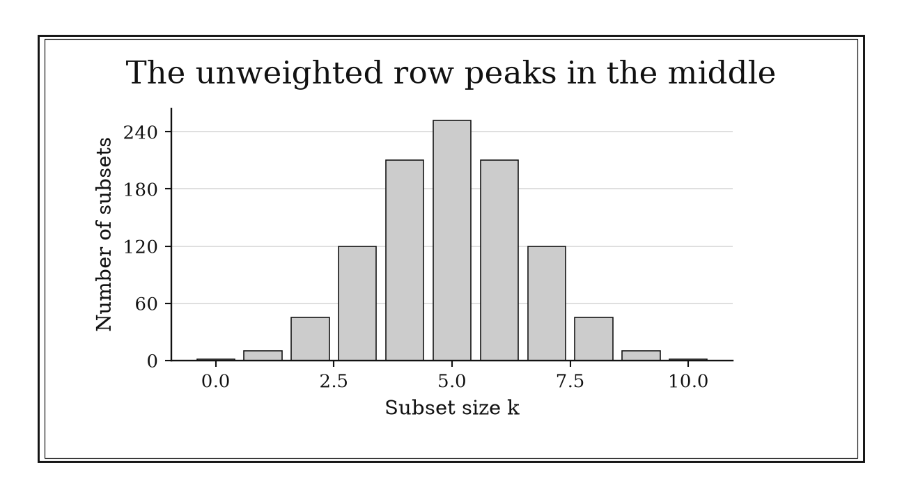
Figure 9.3. For n=10, the binomial row is symmetric and reaches 252 at k=5. Multiplying by unequal probability weights can move the distribution’s peak.
9.3.2: Expect one binary-search step per bit of search space
History
Searching a sorted table one entry at a time could cost nearly as many comparisons as the table had entries, a real expense once computing time itself was scarce and metered. Donald Knuth’s historical survey credits John Mauchly with the first published discussion of a faster approach in 1946: repeatedly checking a middle entry and discarding half the remaining candidates. A fully specified algorithm followed later, with Hermann Bottenbruch publishing a clear version while working in West Germany in 1962. The method itself is the historical artifact; describing its cost as one step per bit of the search space is a modern way of stating the same halving process.
The equation
For integers and , after balanced halvings of candidates, at most
remain. To reduce the candidate set to one, it is sufficient to take
How to read it
Each comparison in a balanced search is a single yes-or-no answer, and a sequence of such answers can only distinguish among different starting positions, since that is how many distinct answer sequences of length exist. So a table of candidates needs roughly comparisons where first reaches , that is, . Doubling the table size adds only one more comparison to that ceiling, the practical meaning of the growth being logarithmic rather than proportional. This describes decision depth under balanced, ordered splitting; it says nothing about the cost of first sorting an unsorted table, which is a separate expense entirely.
How to use it
A university library’s catalog holds 1000 sorted call-number entries, and the systems librarian wants to confirm the lookup algorithm meets its promised worst-case comparison budget before rollout. Since
ten balanced halvings suffice to isolate any single entry, so the librarian sets the comparison budget at ten and confirms the deployed code never exceeds it on the test catalog.
When the catalog grows to 2000 entries after a merger, the ceiling rises to eleven comparisons rather than doubling, since ; one extra comparison is the entire practical cost. Duplicate call numbers would leave a whole range of matching entries rather than a single position, and an unsorted new-acquisitions cart would need its own sorting pass first. This is an Independent rule: under balanced ordered splitting, the number of candidate bits directly predicts search depth.
9.3.3: Estimate derangements by factorial over e
History
The instinct that a full round of the card game Treize would almost always turn up a matching card was wrong, and correcting it required exact enumeration of the opposite case: rounds where no called rank ever matched its card. Montmort worked through that no-match count in the Essay’s second edition, finished by 1713, treating what is now called a derangement. His inclusion-exclusion sum for the no-match count, divided by all possible deals, approaches a fixed limit near 37 percent no matter how large the deck. The nearest-integer shortcut connecting that limit to a whole count is a later mnemonic distilled from Montmort’s alternating sum, not his own phrasing.
The equation
For , the number of permutations with no fixed point is
Because the sum truncates the alternating series for ,
and is the nearest integer to .
How to read it
The exact count of no-fixed-point permutations, written , comes from an alternating inclusion-exclusion sum that, after factoring out , reproduces the first terms of the series for . Because that series alternates and shrinks fast, the fraction of permutations with no fixed points settles near , about , whether is six items or six thousand. The same shrinkage means the leftover error after truncating is less than for , so is the nearest whole number to . The rule assumes every item is barred only from its own position; extra forbidden placements change the calculation.
How to use it
An office holiday party organizer running a gift exchange for 6 participants wants to know how many assignment orders leave nobody drawing their own name, since the game’s fun depends on total mismatch. Dividing , the nearest whole number is 265, also the exact count of fully mismatched assignments out of total orders, so roughly , close to , of random draws already satisfy the no-self-match rule with no adjustment.
The exact alternating sum confirms the estimate rather than approximating it:
A side rule barring certain named pairs from drawing each other, beyond self-draws, would change the inclusion-exclusion structure, and this shortcut would no longer apply directly. This is an Independent rule: for ordinary derangements, factorial over directly gives a remarkably accurate and recoverably exact count.
9.3.4: Estimate multinomial counts on the log scale
History
Writing out the exact number of ways to arrange a mole of particles among energy states would produce a number far too large to print, a wall Ludwig Boltzmann hit in 1877 while working in Vienna on the link between thermodynamic entropy and microscopic arrangement counts. His answer was the logarithm of that multinomial count instead, applying Stirling’s approximation to turn an unmanageable factorial ratio into an expression proportional to entropy. Max Planck later wrote the relationship as . The logarithmic step is Boltzmann’s own move; the entropy notation below is modern.
The equation
Let , let the be nonnegative integers with , and set . For
Stirling’s leading terms give
Here the logarithm is natural and is defined as .
This is a leading logarithmic approximation. For a fixed number of categories as grows, the omitted Stirling remainder is , which is lower order than . If the number of categories grows with , verify that the accumulated remainder is still negligible before interpreting as the dominant scale.
How to read it
is the multinomial count of ways to split items among categories holding of them, each category’s share. Substituting Stirling’s approximation for every factorial cancels the largest terms and leaves times the entropy of those shares, exposing the count’s dominant exponential scale without forming a factorial. Entropy is largest when categories are used evenly and smallest when one swallows nearly everything, so a balanced split produces vastly more arrangements than a lopsided one. The approximation nails the exponential scale but drops smaller square-root correction factors that still matter for exact probabilities.
How to use it
A quality analyst sorting a batch of finished units into two equal categories, pass and rework, wants a quick sense of how many sorting arrangements are possible before an exact audit. With , the entropy is
so the leading scale of the arrangement count is
meaning the count grows like up to a smaller polynomial factor. Since the exact count is , well below the estimate, the analyst treats entropy scale as an order-of-magnitude check, not a substitute for the report’s exact figure.
If the batch instead split unevenly, say 9 units passing and only 1 sent to rework, entropy would drop well below and the arrangement count would shrink to match, a check against a reported sorting count that looks too large for how lopsided the batch was. This is an Independent rule: the log transform directly exposes the dominant scale of multinomial counts across many applications.
9.3.5: Use generating functions to turn convolution into multiplication
History
Casework and cleverness were the only tools for counting outcomes until Euler built a machine that did the bookkeeping for him. Working in St Petersburg in 1741, he represented every partition by the infinite product
Each factor records choosing zero, one, two, or more copies of one particular part size, and the coefficients of the fully expanded product count partitions by total size automatically. This was an original use of the generating-function idea, built to replace repeated case-by-case convolution with one multiplication.
The equation
Let
If , then
How to read it
Write a count as coefficients of a power series, , one coefficient per total size. Multiplying two such series, , produces coefficients , since picking a term from the first series and a term from the second creates one combined outcome of total size , and gathering every such pairing performs the whole convolution at once. The variable never needs to represent an actual quantity or converge to a number; it is a bookkeeping marker for size. Each factor must record exactly one component’s allowed copy counts; getting that encoding wrong, treating labeled and unlabeled components the same way, changes what a coefficient counts.
How to use it
A caterer building boxed lunches wants the number of ways two guests’ independent orders, with each guest choosing a course count uniformly from one through six, could add to a combined total of 7 courses, to plan batch sizes around the most common total. Encoding one guest’s order as
and multiplying two such polynomials, the coefficient of in is , matching the six ordered pairs ; since the two guests are distinguishable, and count as different combined orders, and the kitchen plans batch sizes for six equally likely ways to reach that total.
For a menu item in unlimited quantity, the factor records every copy count of size at once, and multiplying one such factor per item, then reading off coefficient , counts every combination reaching a target total, the structure Euler used for partitions. Mixing up labeled and unlabeled factors would silently change what a coefficient means. This is a Workflow heuristic: it converts repeated coefficient convolution into algebra inside a larger counting method.
9.3.6: Look for Catalan numbers in balanced recursive structures
History
What do a triangulated polygon, a stack of balanced parentheses, and a binary tree’s shape have in common? Euler posed the polygon version between 1751 and 1758, working between Berlin and Halle, asking how many ways a convex polygon could be sliced into triangles. Johann Segner worked out the recursive decomposition, but an arithmetic error corrupted his later values; Euler published a correction restoring the sequence. Only later was it attached to Catalan’s name once mathematicians recognized it recurring in parenthesizations, trees, and balanced paths beyond polygons. The recursive split is historical; calling the pattern a Catalan signal is later recognition.
The equation
With , Catalan numbers satisfy
and
How to read it
In a structure with a first, distinguished split point, such as the side of a polygon touching the first triangle cut from it, everything on one side of the split forms one smaller instance of the same structure, and everything on the other side forms another. If the left piece has smaller units and the right has the remaining , summing over every possible split point produces the defining Catalan recurrence,
An empty side counts as one valid substructure, not zero, which is why and the whole recurrence gets off the ground. The pattern only signals Catalan counting when each object has exactly one such first split; several equally valid first splits need a different recurrence entirely.
How to use it
A construction scheduler needs to confirm how many valid nesting shapes exist for three subcontractor sign-offs, ignoring the subcontractors’ identities, where each inner sign-off must fully close before the one enclosing it does, matching a balanced-bracket structure the scheduling software assumes. Using the closed form for three pairs,
the scheduler confirms exactly 5 valid unlabeled nesting shapes exist, matching what the software’s test suite already expects.
The recurrence offers an independent audit: for four nested pairs,
agreeing with the closed form and confirming the recursive model before the scheduler relies on it for a larger project. If two sign-offs were instead allowed to overlap partway, the balanced-split assumption behind this count would no longer hold. This is a Workflow heuristic: it identifies a recurring recursive family and routes the problem to Catalan formulas or generating functions.
Chapter Synthesis: Count the Structure, Not the Cases
Combinatorics becomes reliable when the notion of an outcome is fixed before enumeration begins.
First identify the direct structure. Pigeonhole turns average load into an unavoidable collision. Independent membership gives . Identical items in labeled unlimited boxes produce stars and bars. Sparse selection permits a falling-product approximation. Overlap calls for inclusion–exclusion, and quotienting by symmetry requires equal orbit sizes.
Then design the workflow. Add disjoint alternatives and multiply staged choices. Decide whether order changes the recorded object. Replace “at least one” with its complement when avoidance is simpler. Build recurrence states from exactly the boundary information future extensions need. Indicators make expectation additive without independence, while double counting proves identities by viewing one incidence set from two sides.
Finally inspect scale and pattern. Adjacent ratios locate the center of a binomial row. Halving makes search depth logarithmic. Inclusion–exclusion makes derangements almost . Logarithms turn multinomial counts into entropy. Generating functions multiply independent size contributions, and Catalan recurrences reveal balanced noncrossing structures.
Across all eighteen rules, ask four questions:
- What exactly makes two outcomes the same or different?
- Are choices alternatives, stages, restrictions, or symmetries?
- Does the rule return the count, or prepare a larger counting method?
- What assumption, independence of choices, uniform orbit size, sufficient state, or asymptotic scale, makes the shortcut valid?
One-Page Combinatorics Toolkit
| Recognition cue | Rule to try | What it gives | Role |
|---|---|---|---|
| More objects than category capacity | Ceiling pigeonhole | Guaranteed occupancy | Independent |
| Unrestricted membership in an -set | Two choices per element | subsets | Independent |
| Identical items, labeled unlimited boxes | Stars and bars | Exact distribution count | Independent |
| Small selected from large | Sparse-selection estimate | Independent | |
| Two overlapping alternatives | Subtract the intersection | Exact union count | Independent |
| Objects equivalent under symmetry | Verify uniform orbit size before division | Quotient count | Independent |
| Disjoint alternatives or staged choices | Sum across, multiply along | Counting architecture | Workflow |
| Selection versus arrangement | Ask whether swapping changes the outcome | Combination or permutation route | Workflow |
| “At least one” has an easy opposite | Count the complement | Simpler equivalent count | Workflow |
| Restricted object built one step at a time | Preserve future-relevant state | Valid recurrence | Workflow |
| Count inside a random object | Sum indicators | Expected count | Workflow |
| Two expressions may count one pair set | Double-count incidences | Combinatorial identity | Workflow |
| Need the largest unweighted binomial term | Inspect adjacent ratios | Central maximum | Independent |
| Ordered search halves candidates | Count bits of search space | Logarithmic depth | Independent |
| Permutation forbids every fixed point | Use | Derangement estimate or exact rounding | Independent |
| Huge multinomial coefficient | Take logs and use entropy | Exponential scale | Independent |
| Additive sizes combine repeatedly | Multiply generating functions | Convolution by coefficients | Workflow |
| Balanced, rooted, noncrossing split | Test a Catalan recurrence | Catalan family route | Workflow |
Decision Path
- Can the answer be forced without enumeration? Define boxes and try pigeonhole, or identify unrestricted binary membership.
- Are identical units being distributed? Use stars and bars only when recipients are labeled and capacities are unlimited.
- Are several cases being combined? Add disjoint alternatives, multiply staged choices, and subtract intersections when alternatives overlap.
- What makes outcomes distinct? Decide whether order matters and whether rotation, reflection, or another symmetry identifies descriptions.
- Is a restriction awkward? Count its complement, or design recurrence states that remember precisely what legal extension depends on.
- Is the object random? Express the target count as indicators before trying to analyze dependencies.
- Is an identity the goal? Define one incidence set and count it in two orders.
- Is the exact count enormous? Use adjacent ratios, logarithms, or a regime-appropriate approximation to expose scale.
- Does the construction split recursively or add component sizes? Look for Catalan structure or encode the components with a generating function.
Transfer Problems
1. Define the outcome before choosing a formula
Ten people are available. Compare the number of three-person committees, the number of committees with a designated chair, and the number of ordered first–second–third speaking schedules. For each count, state whether order matters and identify any uniform overcounting factor.
2. Replace restrictions with structure
Count binary strings of length eight that contain at least one . Then design two recurrence states for length- binary strings containing no consecutive s, derive their transitions, and compute the total for . Explain why the complement shortcut solves the first restriction but not the second by itself.
3. Recognize scale and recursion
For a balanced-parenthesis string with four pairs, derive the first-object split and compute the count from the Catalan formula. Then compare that count with all unrestricted parenthesis-like binary strings and explain how equal opening and closing totals, together with nonnegative balance at every prefix, remove the others.
Where These Ideas Reappear
- Probability: complements, indicators, binomial coefficients, and derangements turn counts into event probabilities and expectations.
- Graph theory: pigeonhole, double counting, and recurrence states become degree bounds, incidence identities, and path algorithms.
- Algorithms: binary search, dynamic programming, and generating functions translate combinatorial structure into running time and computation.
- Number theory: pigeonhole controls residues and rational approximation, while generating functions encode partitions.
- Statistical mechanics and information theory: multinomial multiplicity becomes entropy on the logarithmic scale.
- Algebra: group actions, orbits, and stabilizers determine when symmetry division is legal.
- Asymptotics: sparse binomial estimates, , Stirling’s formula, and central coefficients reveal dominant scale without exact arithmetic.
Historical Notes and Sources
Every rule in this chapter has a verified historical connection. The modern formulas, notation, and decision-language remain operational interpretations of the documented events.
- Dirichlet and pigeonhole: Historical study of pre-Dirichlet pigeonhole uses; survey of Dirichlet approximation.
- Pingala and binary prosody: Scholarly study of Pingala’s combinatorial algorithms.
- Bose and indistinguishable occupation counts: Historical study of Bose’s 1924 derivation.
- Poisson and rare-event counting: Historical remarks on the Poisson distribution.
- Montmort, coincidences, and derangements: Montmort’s 1713 Essay d’analyse sur les jeux de hazard; MacTutor on Montmort and Treize.
- Pólya and chemical symmetry: Pólya’s 1937 enumeration paper.
- Pascal, Fermat, and gambling enumeration: American Physical Society history of the 1654 correspondence.
- Bellman and dynamic-programming states: Bellman’s 1954 paper; INFORMS biography.
- Erdős and indicator counting: Historical survey of the probabilistic method; Stanford notes on the first-moment Ramsey proof.
- Euler and bridge incidences: Euler Archive, Königsberg paper; English translation.
- De Moivre and central binomial behavior: MacTutor biography of Abraham de Moivre.
- Binary search: Knuth’s historical notes on searching.
- Boltzmann and multiplicity: American Physical Society history of statistical entropy; translation and commentary on Boltzmann’s 1877 paper.
- Euler and generating functions for partitions: Euler Archive, De partitione numerorum; English translation.
- Euler, Segner, and Catalan numbers: Igor Pak, “History of Catalan Numbers”; MAA primary-source project on triangulation counts.
- Modern combinatorics statements: Joy Morris, Combinatorics; Lehman, Leighton, and Meyer, Mathematics for Computer Science. These sources support the modern mathematics, not the exact historical phrasing of the rules.