Chapter 10: Graph Theory: Structural Tests for Networks
A network diagram invites motion. Trace a route, try a coloring, assign partners, or launch a shortest-path algorithm. But many graph problems are decided before any search begins. Ninety edges cannot connect one hundred vertices. Four odd-degree vertices make an edge-by-edge tour impossible. Ten edges force beyond the planar limit. Four applicants sharing only three possible jobs cannot all be assigned.
These are obstruction tests: small pieces of structural evidence that certify what a graph can or cannot do. They save work because they replace a search through arrangements with a count, parity condition, or neighborhood inequality.
The ten rules in this chapter form three families. The first extracts global information from vertices and edges. The second searches for decisive obstructions to bipartitions, planar drawings, and matchings. The third chooses traversal and construction methods only after checking the assumptions that make them valid.
The governing habit is: before running an algorithm on a network, ask what its counts, degrees, cycles, and neighborhoods have already proved.
10.1: What Edge Counts Reveal
An edge is local, but counting all edge ends reveals global restrictions. The handshaking identity fixes average degree. The threshold rules out connectedness when the edge budget is too small. Combined with one additional condition, the same count certifies a tree.
10.1.1: Use handshaking to convert edges into average degree
History
Get the bridge count wrong by even one and the whole puzzle changes. Between 1735 and 1741, Euler reduced Königsberg to four landmasses and seven bridges, setting aside every fact except how many bridge ends touched each landmass: not length, shape, or arrangement, just the count. That reduction was the discovery. Euler’s own argument turned on parity, odd or even, not on an average; treating the same double count as an average degree is a later reading of his method, not his own language. The payoff was permission to reason about connections without ever drawing a map.
The equation
For a finite undirected graph ,
Therefore the average degree is
How to read it
Every plain edge has two ends, one at each vertex it touches. Add every vertex’s connection count and each edge has been counted twice, so the total is always double the edge count. Divide by the number of vertices for the average connections per vertex.
Averages force existence: at least one vertex sits at or above that average and one at or below it, the same logic behind a class average. What the average will not tell you is the spread: one highly connected hub surrounded by loners can share an average with a network where every vertex looks alike.
How to use it
A community platform’s moderator is told a 20-member interest group has 50 mutual-connection links, and a member complains that nobody in the group has more than 4 connections. The moderator does not need to open the friend graph:
Average degree is , so at least one member must have connections or more, and the complaint is false on its face.
Because the degree sum is always even, the number of odd-degree members in this connection graph is even too, a parity check she reuses when screening whether a route can traverse every connection exactly once (Rule 10.3.1).
What the number alone will not reveal is who the well-connected members are, or whether ties cluster around one hub or spread evenly; a hub-and-spoke group and a uniformly friendly one can post the same average. She confirms the platform tracks mutual, not one-way, connections before trusting the figure. This is an Independent rule: it turns two basic counts into a reusable density and degree certificate.
10.1.2: Use n-minus-one as the connectedness edge floor
History
No rerouting trick can make a network connected if it is missing links below a hard floor. In 1926, Otakar Borůvka worked on joining every site in Moravia to an electric grid as cheaply as possible, minimizing the total line length built. Beneath that optimization sat a plainer fact: any design connecting every site needs at least one fewer line than there are sites. Borůvka’s procedure chases the cheapest such design, but the floor does not care about cost or geography, letting an engineer reject an underbuilt plan by counting alone.
The equation
For a finite connected undirected graph,
Equivalently,
How to read it
Picture every site starting alone and unlinked, as many separate pieces as there are sites. Each new connecting line merges at most two pieces into one, so joining everything into a single piece takes at least one line fewer than the site count; joining 10 scattered stepping stones into one path takes at least 9 planks. The same floor falls out of a different fact: any connected network contains a spanning tree using exactly that many lines. The floor is silent on whether the lines actually connect everything: the same total can sit bunched inside one crowded cluster while other sites stand isolated.
How to use it
A rural utility is scoping a plan to connect 100 substations to the grid, and the budget office has approved only 90 line segments. Before the engineer drafts a single route, the floor rules the plan out:
so no arrangement of 90 lines can connect all 100 substations, however cleverly they are drawn. She sends the plan back for more line budget rather than reworking the layout.
The reverse deduction is dangerous: reaching 99 lines removes the floor’s veto but does not certify a working network, since 99 lines could still bunch inside one cluster while others sit unreached. Confirming the network is connected still needs a separate layout check, and a backup route for one line failing needs budget above the bare floor. This is an Independent rule: a deficient edge count alone gives a complete nonconnectedness certificate in any application modeled by an undirected network.
10.1.3: Recognize a tree by the n-minus-one edge count plus one condition
History
Chemists could sketch several branching patterns for a given carbon count without being sure they had found every one, or ruled out an impossible one, for the formula . In 1874 and 1875, Arthur Cayley settled that uncertainty by treating each candidate skeleton as a graph: carbon atoms became vertices, bonds became edges, and a valid skeleton had to be connected and cycle-free, a tree. Chemical valence added its own constraints, but the graph decided which branching patterns could exist at all.
The equation
For a finite undirected graph with and , any two of the following conditions imply the third:
In particular, every tree satisfies
How to read it
Start with one carbon and add carbons one at a time; each arrives with exactly one new bond attaching it to the growing skeleton, the way a new employee joins an org chart through one reporting line. After atoms, that growth rule has used exactly bonds. The same count runs both ways: a connected skeleton with more bonds must contain a loop, and one with fewer cannot be fully connected, so any two of connected, loop-free, and bond count pin down the third. Bond count alone, without connectedness or loops, proves nothing.
How to use it
A logistics planner reviews a proposed distribution network of 12 regional hubs linked by 11 direct routes, already known to be connected end to end. Since and the network is connected, it must be a tree: every route is a bridge, exactly one path connects any two hubs, and losing a single route splits the network. The planner flags this as a fragility warning, not praise.
The count alone would not have been enough: a triangle of three hubs plus one hub with no route to it also has and , yet is disconnected and cyclic, not a tree. Pairing the edge count with a separate check, connected or acyclic, whichever is cheaper to verify, settles the question. This is an Independent rule: the edge count plus connectedness or acyclicity directly certifies tree structure across networks, hierarchies, and molecular skeletons.
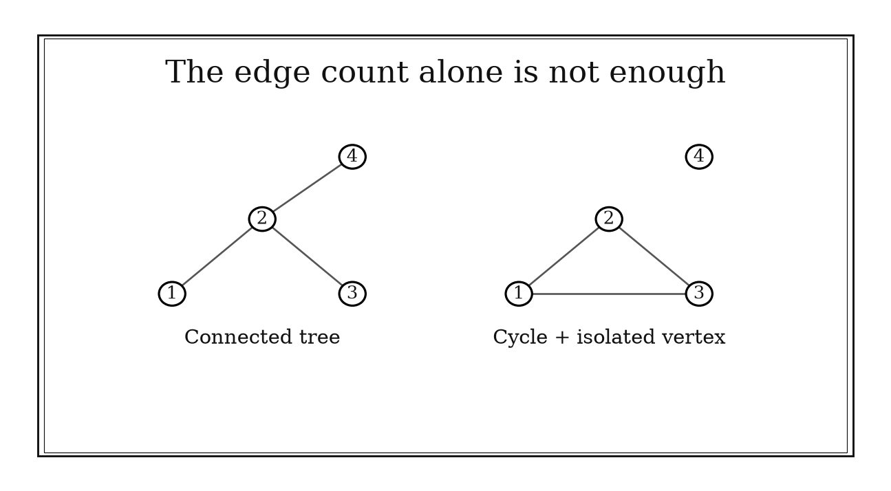
Figure 10.1. Both drawings have four vertices and three edges. Only the connected drawing is a tree; a triangle plus an isolated vertex has the same count but contains a cycle.
10.2: Fast Obstruction Tests
Some graph properties are hard to construct but easy to disprove. An odd cycle blocks a two-class split. Too many edges block planarity. A subset with too few neighbors blocks a full matching. In each case, a small witness ends a much larger search.
10.2.1: Test bipartiteness by searching for an odd cycle
History
Can every worker in a two-shift rotation be paired off so that no one shares a shift with a conflict? Dénes Kőnig’s 1936 book gave graph theory its first systematic treatment, and within it he built out the theory of graphs whose vertices split cleanly into two classes. The surviving record favors this broad synthesis over one dramatic discovery moment. His name still anchors the foundational results on matching within such two-class graphs. The odd-cycle test that answers the pairing question renders the same structural idea as a decisive check rather than a whole theory.
The equation
A graph is bipartite when its vertices can be partitioned as
so that every edge has one endpoint in each part. Equivalently,
How to read it
Picture assigning each vertex to one of two teams by walking outward from a start point, switching teams with every step along a path. Returning to the start after an even number of steps fits a two-team split; an odd number is only possible if some path forced a vertex onto both teams at once. That contradiction is an odd cycle, the only way a two-team split can fail. Coloring must be redone separately in each disconnected piece of a network. The test cannot certify internal team compatibility, only whether the two-way split itself can hold.
How to use it
A charge nurse is building a two-team handoff schedule and draws a conflict edge between any two staff members who cannot share a team, based on overlapping certifications or reporting lines. Three staff members conflict with each other pairwise: and all pairs conflict, forming a triangle. Assign the first to team A and the second, forced by conflict, to team B; the third conflicts with both and cannot join either team. That triangle alone certifies the schedule is impossible.
She checks each ward separately, since one ward’s conflicts say nothing about another. If certifications instead impose one-directional restrictions, a senior staffer covering a junior’s shift but not the reverse, the plain two-coloring model no longer applies and a directed scheduling model is needed instead. This is an Independent rule: it characterizes bipartite structure and produces a transferable obstruction witness.
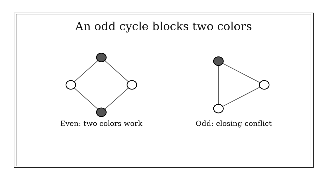
Figure 10.2. Alternating two vertex colors works around an even cycle. On the triangle, the closing edge joins two vertices assigned the same color, certifying failure.
10.2.2: Use the planar edge bound as a quick nonplanarity screen
History
A convex solid hides an arithmetic relation among its corners, edges, and faces. Between 1750 and 1758, Euler tested that relation, , across families of polyhedra, seeking an invariant that survived every shape. Flatten one face onto a plane and the skeleton becomes a planar graph. Euler’s formula belongs to that solid-geometry search; the compact edge ceiling is a later deduction from his invariant, not a claim he made himself, but it is what lets a modern reader reject an impossible flat drawing with one line of arithmetic instead of a hunt through diagrams.
The equation
For a simple planar graph with vertices and edges,
If a planar embedding has every face boundary of length at least four, as in a simple bipartite planar graph, then the stronger bound is
How to read it
A crossing-free drawing divides the page into regions; corners minus connections plus regions equals two. Every region uses at least three connection-sides and every connection borders two regions, so three times the regions is at most twice the connections. That combination removes the region count, leaving a ceiling on connections from corners alone. In practice the ceiling allows just under three connections per corner: 100 corners cap at connections, so a dense web on few corners is the first suspect. It only works one way: too many connections proves no flat drawing exists, but staying under it proves nothing by itself.
How to use it
A circuit board designer is checking whether a trace layout with 5 pads and all 10 possible pairwise traces can be etched on one layer without crossings. The ceiling for pads is traces, and the design calls for , one more than allowed. No arrangement of those 10 traces avoids a crossing, so the extra connection routes to a second layer.
A second layout, 6 pads with 9 traces and no triangular groupings, passes that basic test but is still suspect: layouts with no three-sided regions need the tighter ceiling , and 9 exceeds it, so this one too needs a second layer. Passing either ceiling is not a green light; a board with few traces can still turn out unroutable once layer rules are added. This is an Independent rule: an excess edge count conclusively rejects planarity across circuit, map, and network models.
10.2.3: Check Hall bottlenecks before seeking a perfect matching
History
Whether a full assignment is possible, or doomed by a single overcommitted subgroup, was the exact stake behind Philip Hall’s 1935 theorem on systems of distinct representatives, published in the Journal of the London Mathematical Society while he worked at King’s College, Cambridge. Given a family of finite sets, Hall asked whether every set could get its own distinct representative, none shared. The later marriage-theorem language recasts sets as people and representatives as acceptable partners, a vivid retelling, but Hall’s mathematics concerned sets, not romance. Failure is always traceable to one collectively overcommitted group.
The equation
For a bipartite graph , there is a matching that covers every vertex of exactly when
where is the set of right-side neighbors of vertices in .
If , such a matching is perfect.
How to read it
Take any cluster on the side needing full coverage, and count how many distinct options it can reach between its members. More members than reachable options guarantees some member is left unmatched, the pigeonhole logic that puts two letters in one mailbox when there are more letters than boxes. What makes the rule powerful is the reverse: if no cluster ever comes up short, a full assignment for the entire side is guaranteed to exist. Checking members one at a time can miss a cluster that only runs short once several overlap the same narrow options.
How to use it
A school registrar is finalizing elective placements and finds that four students have each requested only sections that, between them, cover just three available elective slots. Let be those four students; their reachable slots form with
so Hall’s condition already fails. No rearrangement of the schedule can seat all four in a slot of their own; one is bumped to a different course, and the registrar tells that family before the term starts.
Checking eligibility one student at a time misses this: each might qualify for two or three sections, yet collectively fall back on the same narrow set of three. For a handful of students, scanning overlapping subsets by hand is enough; for a full school’s schedule, a matching or flow algorithm finds a complete placement or the exact bottleneck group. This is an Independent rule: it gives a necessary-and-sufficient structural criterion and a broadly useful impossibility certificate.
10.3: Traversal and Construction Choices
Once simple obstructions have been checked, an algorithm may be appropriate. Degree parity decides whether an edge-covering trail can exist. Maximum degree gives a safe coloring ceiling. Edge costs determine whether breadth-first search or Dijkstra’s method has the correct shortest-path guarantee.
10.3.1: Count odd-degree vertices before seeking an Euler trail
History
No one in Königsberg crossed all seven bridges exactly once, though residents wondered whether such a route existed. Reducing each land area to a point linked by its bridges, Euler counted four points with an odd number of links, and that single count settled the question: a walk can tolerate at most two such points, so four ruled out every possible route across the city before anyone tried one. It remains the archetype for stopping a search with one small count instead of exhausting every path by hand.
The equation
For an undirected graph whose edge-bearing vertices lie in one connected component:
and
How to read it
Walk through any street on a route and you use one connection to arrive and a different one to leave, pairing up two connections at that intersection each time. Only the first and last intersections may keep one connection unpaired, so only they may show an odd count. If every intersection is even, a route can start and end at the same place; exactly two odd means any route must start at one and end at the other; any other odd count rules the route out. What the count alone will not settle is whether the streets form one connected network; a cut-off segment breaks the guarantee regardless of parity.
How to use it
A public works planner wants a snowplow to clear every street in a neighborhood in one pass, crossing each segment exactly once. She counts how many segments meet at each intersection: four turn up with an odd count, the same pattern the Königsberg bridges gave Euler, so she stops: no single-pass route exists, and splitting the plow route into two trips is unavoidable.
A neighboring district has exactly two odd-count intersections. There a one-pass route is possible, but only starting at one of those two and ending at the other; starting anywhere else guarantees a segment gets missed or repeated. The count only works if every street-bearing intersection sits in one connected network, and it covers segments once each, not intersections once each, a different and harder request. This is an Independent rule: it directly decides existence for an entire class of route problems before construction begins.
10.3.2: Use maximum degree plus one as a greedy coloring ceiling
History
Give every conflicting pair of values a different register, and a compiler never overwrites a value still in use. In 1981 and 1982, Gregory Chaitin and colleagues at IBM Research built exactly that model: values alive at the same moment became adjacent vertices in an interference graph, and machine registers became colors. Their experimental PL/I compiler approached hand-tuned performance, and later versions added spilling, moving a value to memory when registers ran short. The sophistication was in the ordering and spilling strategy; the coloring ceiling underneath is a simpler guarantee that any conflict graph can always be colored with enough registers to go around.
The equation
For a finite loopless graph with maximum degree ,
The basic greedy algorithm processes vertices in any order and gives each vertex the first color not used by an already colored neighbor.
How to read it
Count the busiest vertex’s connections across the network and call that number . Color vertices one at a time, giving each the first unused color among its already-colored neighbors. No vertex can be blocked, since it has at most neighbors, so at most colors are ever off-limits, leaving one free among choices, the way a table set for one more place than the busiest guest’s list of conflicts always seats everyone. This only guarantees enough colors exist; the fewest actually needed stays open, since the coloring order can change it a great deal.
How to use it
A tournament scheduler assigns time slots to matches, drawing an edge between any two that share a team, court, or referee and so cannot run together. No match in this bracket conflicts with more than others, so slots are opened, and matches are colored greedily in scheduling order, each taking the first open slot not used by a conflicting match. Every match is guaranteed a slot, since none can face more than 4 taken conflicts out of 5 options.
Even inside this bracket, a good ordering can finish in fewer than 5 slots; the ceiling is a guarantee, not an estimate. The scheduler treats 5 as a safe fallback, not a target, and tries to shrink it first. This is an Independent rule: it supplies a constructive, application-wide ceiling whenever a safe coloring matters more than an optimal one.
10.3.3: Use breadth-first search for unweighted shortest paths
History
Intuition said a shortest route through a maze could only be found by trying enough candidate paths to be sure none did better. Edward F. Moore’s 1959 paper The Shortest Path Through a Maze disagreed: flood every position one step from the start, then two steps away, continuing outward in layers until the destination surfaces. Reaching the exit first in a given layer proved no shorter route existed, since every shorter distance had already been explored. It replaced trial-and-error maze running with a guarantee depending only on discovery order, not which routes were tried.
The equation
For an unweighted graph and source , breadth-first search assigns a level satisfying
With adjacency lists, its running time is
How to read it
Starting from one point, mark everything reachable in one move as layer one, then everything newly reachable as layer two, and so on outward. A first-in, first-out queue guarantees every position in one layer is found before any in the next, so a location’s layer number is exactly its shortest distance in moves from the start, the same guarantee a rippling wave gives about which shore it reaches first. Tracing back to the neighbor that first discovered a position retraces an actual shortest route. This depends on every move costing the same; once costs differ, layer number stops matching true distance.
How to use it
A warehouse operations lead checks whether a picking robot’s proposed route between two shelving bays is shortest, given every aisle move costs the same one unit. Starting the layer expansion from the robot’s bay, its target first appears in layer 4, so a four-move path exists, and no route of three or fewer moves can exist, since layers 0 through 3 were fully searched first. The lead accepts the four-move route without checking alternatives by hand.
If a redesign adds a slow conveyor shortcut that takes longer to cross than a normal aisle step, the equal-cost assumption breaks: a four-move route through it could lose to a five-move route avoiding it. Once aisle costs differ, the lead needs Rule 10.3.4 instead. This is a Workflow rule: it is the appropriate shortest-path stage only after the edge-cost model has been classified as unweighted or equal-weight.
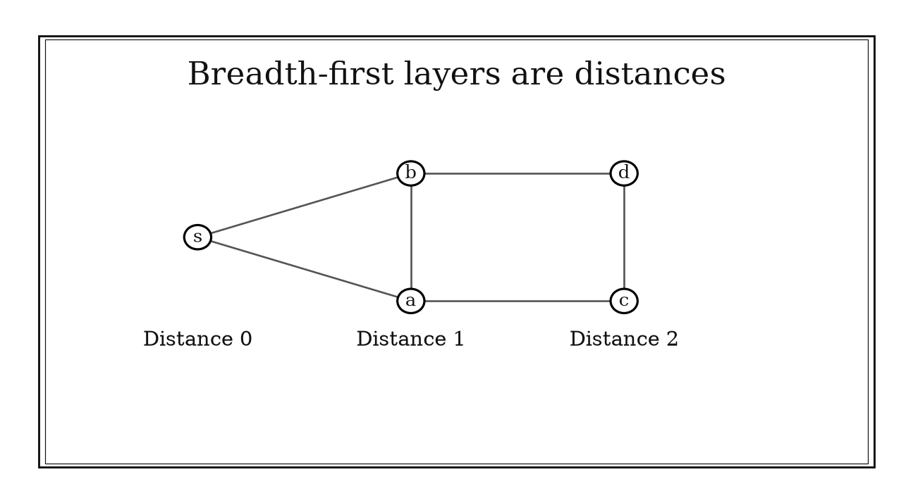
Figure 10.3. With unit-cost edges, first discovery in layer two certifies distance two from the source. The extra edge within layer one does not create a shorter route to layer two.
10.3.4: Use Dijkstra only with nonnegative edge weights
History
How do you find the cheapest route across a map without checking every possible path? Edsger Dijkstra faced that exact demonstration problem preparing a show for the ARMAC computer in Amsterdam. He later recalled picking a map problem and working out the core idea in about twenty minutes; the formal paper followed in 1959. His method permanently settles the smallest tentative distance found so far and never revisits it. That shortcut is only sound when adding another road segment can never make a route cheaper, exactly what Dijkstra’s original proof assumed.
The equation
Given source , relaxation updates an edge by
Dijkstra’s settling proof requires
How to read it
At each step, the method locks in whichever unfinished location currently has the smallest known travel cost, reasoning that any other route reaching it later can only cost the same or more once another leg’s cost is added. That reasoning depends entirely on every leg costing zero or more. A negative-cost leg breaks it completely: a route that looked expensive at its first stop can pick up a large discount further along, arriving cheaper than a route the method already locked in and moved past.
How to use it
A travel planner is comparing flight-cost routes on a network where costs , costs , and a promotional credit turns into a rebate worth . Running the settling method in order, looks cheapest first at cost and gets locked in immediately. But the route totals , cheaper than the already locked in, and the method has already moved past .
The planner cannot fix this by re-running the algorithm more carefully; the rebate leg invalidates the method’s core guarantee, and a different approach for negative legs is needed whenever a promotional credit or refund appears in the cost network. Ordinary zero-cost legs, like a free connecting shuttle, cause no trouble. Once every leg costs zero or more, the settling method resumes giving an efficient, guaranteed-correct answer. This is a Workflow rule: it guards algorithm selection inside a larger shortest-path calculation.
Chapter Synthesis: Inspect Structure Before Search
Graph theory often turns a global question into a small certificate. Handshaking converts an edge count into average degree and parity information. The threshold rejects underconnected networks and, with connectedness or acyclicity, recognizes trees. Odd cycles, excess planar edges, and Hall-deficient subsets expose impossibility without enumerating arrangements.
Algorithms enter only after the model is classified. Degree parity decides whether an Euler trail is worth constructing. Maximum degree supplies a safe greedy color budget. Equal edge costs point to breadth-first search; unequal nonnegative costs point to Dijkstra. A negative weight is not a minor numerical detail, it removes the proof that makes Dijkstra’s settled distances final.
Across all ten rules, ask four questions:
- What do vertex, edge, and degree counts force before any search?
- Is there a small cycle, subset, or inequality that certifies impossibility?
- Does the desired route concern edges, vertices, assignments, or path cost?
- Which graph and weight assumptions make the selected algorithm correct?
One-Page Graph Theory Toolkit
| Recognition cue | Rule to try | What it gives | Role |
|---|---|---|---|
| Vertex and edge counts are known | Compute | Average degree and degree existence bounds | Independent |
| A graph may be connected | Compare with | Fast disconnection certificate | Independent |
| Tree structure is suspected | Combine with connectedness or acyclicity | Tree certificate | Independent |
| Vertices must split into two conflict-free groups | Two-color and search for an odd cycle | Bipartition or obstruction | Independent |
| A network is claimed to be planar | Check , or when applicable | Fast nonplanarity certificate | Independent |
| Every left-side item needs a distinct partner | Check | Matching criterion or bottleneck | Independent |
| Every edge must be used once | Count odd-degree vertices and check connectivity | Euler-trail decision | Independent |
| A safe coloring ceiling is enough | Greedily use at most colors | Constructive upper bound | Independent |
| Every edge has equal cost | Run BFS | Shortest paths in edge count | Workflow |
| Edge costs are unequal but nonnegative | Run Dijkstra | Weighted shortest paths | Workflow |
Decision Path
- Are only and known? Compute average degree and compare the edge count with . These may settle the question before adjacency data is inspected.
- Is a graph at the threshold? Verify either connectedness or acyclicity. The count alone does not prove it is a tree.
- Is the desired split binary? Two-color each component. A conflict should be reported with its odd-cycle witness.
- Is a planar drawing requested? Apply the appropriate edge ceiling first. Failure proves nonplanarity; success merely permits further testing.
- Is the task a one-to-one assignment? Model a bipartite graph and look for a subset whose neighborhood is too small before attempting exhaustive assignments.
- Must every edge be traversed once? Count odd degrees and check connectivity among edge-bearing vertices. Do not confuse the task with visiting every vertex once.
- Is a coloring required? Decide whether a guaranteed construction is sufficient or optimization is worth the additional effort.
- Is the task shortest path? Equal costs suggest BFS. Unequal nonnegative costs suggest Dijkstra. Any negative weight requires a different correctness argument.
Transfer Problems
1. Diagnose a proposed network from counts
A simple graph has vertices and edges. What can you conclude about connectedness? Now suppose a different graph has vertices, edges, and is known to be connected. What additional structure follows? Explain why the edge count alone would not support the second conclusion.
2. Find the obstruction before constructing
A bipartite assignment model has five workers on the left. Three particular workers collectively can perform only two jobs, although every worker individually has degree at least two. Identify the relevant Hall set and state the conclusion. Then explain why checking minimum degree alone misses the obstruction.
3. Route three path problems correctly
Choose the first test or algorithm for each case: an undirected street graph in which every street counts as one hop; a road network with nonnegative travel times; and a currency-exchange graph whose transformed edge weights may be negative. State why BFS, Dijkstra, or a negative-weight method is justified in each case, and distinguish a shortest-path task from an Euler-trail task.
Where These Ideas Reappear
- Combinatorics: handshaking, face boundaries, and Hall’s condition are double-counting and pigeonhole arguments in graph form.
- Linear algebra: adjacency, incidence, and Laplacian matrices translate degree and connectivity structure into spectra and null spaces.
- Optimization: spanning trees, matchings, coloring, and shortest paths turn structural constraints into discrete optimization models.
- Computer science: BFS, Dijkstra, register allocation, dependency analysis, and network routing are direct implementations of these rules.
- Chemistry: molecular skeletons use graph connectivity, degree, cycles, and tree enumeration.
- Operations research: assignment bottlenecks and capacity extensions lead from Hall’s theorem to flows and transportation models.
- Topology: Euler’s planar invariant links embeddings and surfaces to combinatorial counts.
- Data and social networks: average degree, bipartitions, distances, and components summarize large relational systems before detailed modeling.
Historical Notes and Sources
The profiles use documented mathematical events and applications, while distinguishing later operational interpretations such as the average-degree consequence and the elementary coloring ceiling.
- Euler, Königsberg, degree parity, and handshaking: Euler Archive, original Königsberg paper; English translation of Euler’s paper.
- Borůvka and economical network connection: historical translation and analysis of Borůvka’s 1926 algorithm; NIST Dictionary of Algorithms.
- Cayley and chemical trees: historical review, “The Chemical Applications of Graph Theory”.
- Kőnig and bipartite graph theory: study of Kőnig’s bipartite characterization and its 1936 source.
- Euler’s polyhedron formula and planar graphs: MAA investigation from original sources; Historia Mathematica note on Euler’s polyhedron articles.
- Hall’s matching theorem: London Mathematical Society historical survey; open manuscript of the survey.
- Graph coloring in register allocation: IBM Research, “Register allocation via coloring”; IBM Research, “Register allocation & spilling via graph coloring”.
- Moore and breadth-first maze search: bibliographic record for The Shortest Path Through a Maze; publication record for Moore’s 1959 paper.
- Dijkstra and nonnegative shortest paths: CWI repository, Dijkstra’s 1959 paper; CWI history of Dijkstra and the ARMAC demonstration.
- Modern graph-theory methods and conventions: Joy Morris, Basics of Graph Theory; Lehman, Leighton, and Meyer, Mathematics for Computer Science.