Chapter 11 , Asymptotics: Finding What Matters at Scale
For a long practical interval, (n^{100}) can be larger than (2^n). Eventually the exponential wins by an overwhelming margin. Both statements are true because “grows faster” is not a claim about every input. It is a claim about what survives when the controlling parameter becomes large.
Asymptotics is the mathematics of disciplined neglect. It identifies a regime, ranks competing terms, retains enough information for the requested accuracy, and proves, or at least clearly labels, what has been discarded. Used well, it turns enormous factorials into logarithms, discrete sums into integrals with corrections, and concentrated integrals into local Gaussian calculations. Used carelessly, it erases the very term a subtraction was meant to reveal.
The fourteen rules in this chapter form three families. The first finds the governing regime and transition scale. The second supplies portable estimates for factorials, harmonic sums, monotone sums, shrinking tails, products, and error orders. The third prevents invalid asymptotic algebra and identifies when specialized summation or saddle methods are justified.
The governing habit is: name the limiting regime, expose its dimensionless parameter, and retain terms through the first order that can change the answer.
11.1: Regimes and Dominant Behavior
Before expanding anything, decide which parameter moves, in what direction, and which terms can compete. A hierarchy ranks familiar growth classes. Dominant balance locates crossovers. Dimensionless ratios make “small” and “large” independent of the units used to describe them.
11.1.1: Use the log-power-exponential growth hierarchy
History
Claim that exponentials always beat powers, and the arithmetic disputes you for a long stretch of ordinary inputs: a modest power can outrun a modest exponential well past any hand-computed range. G. H. Hardy took that dispute seriously, writing Orders of Infinity in 1910 in Cambridge, building on Paul du Bois-Reymond’s comparisons of functions and the order notation of Bachmann and Landau, organizing unbounded quantities into a hierarchy where one growing function eventually becomes negligible beside another.
The equation
For fixed constants (a,p,c>0), as (n),
and
Here (f=o(g)) means (f(n)/g(n)).
How to read it
Each comparison says which quantity eventually swamps the other; it does not settle which is bigger at any one finite input. A power of the logarithm is dwarfed by any fixed power of (n), dwarfed by any exponential with positive rate, dwarfed by the factorial, whose growth accelerates as each factor grows a full unit larger.
Think of a staggered race: the logarithm and power finish while the exponential is still leaving the lot, yet far down the track the exponential and factorial lap everything. The hierarchy guarantees an eventual order but leaves the crossover point unnamed; direct calculation alone locates it, with every exponent and base fixed.
How to use it
A shipment-routing engine has two candidate algorithms: Algorithm A scales like (n^3) microseconds, Algorithm B like (1.1^n), where (n) counts distribution zones. At (n=60): (60^3=216{,}000) versus (1.1^{60}e^{5.72}), so B looks like the winner. But a fixed power is eventually negligible beside any exponential, so B must overtake A eventually; at the five-year cap, (n=120): (120^3=1{,}728{,}000) against (1.1^{120}000), still a win, so the analyst adopts B.
The crossover sits somewhere in the 150-to-170 zones, outside the plan but close enough that a later round should not assume the same ranking. This is an Independent rule: once the regime and fixed parameters are stated, it directly ranks broad classes of growth across algorithms, series, and models.
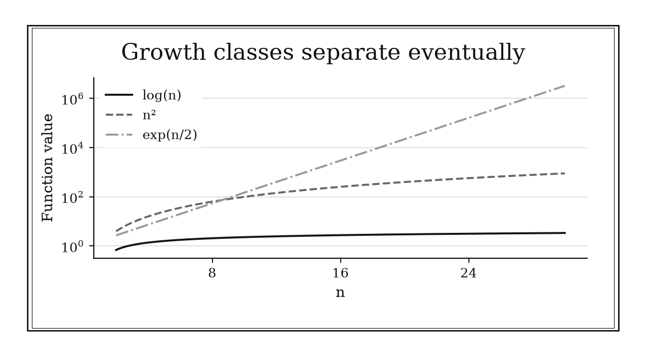
Figure 11.1. These fixed functions illustrate logarithmic, quadratic, and exponential growth. Their order at a finite input depends on constants; the eventual hierarchy does not locate a practical crossover.
11.1.2: Balance competing terms to find the transition scale
History
A fluid with almost negligible viscosity still exerts drag against a solid wall, and explaining why required comparing terms rather than dropping the small one. At the International Congress of Mathematicians in Heidelberg on August 12, 1904, Ludwig Prandtl presented an answer: away from a wall, viscosity is negligible, but inside a thin boundary layer, velocity changes so sharply the viscous term rivals inertia, a documented use of dominant balance: equate two competing effects to find the region where neither can be dropped, locating a transition scale before solving the full equations.
The equation
To compare terms
set their magnitudes equal. When (A,B>0) and (pr),
Equivalently, the ratio of the two terms is order one at the transition.
How to read it
Picture two competing effects, each a coefficient times a power of a variable, one carrying a small parameter. Far from the crossover, one term alone controls the answer, the dominant, or leading, term; near the crossover the sizes become comparable and neither can be discarded. Setting the magnitudes equal gives the transition scale, where control passes from one mechanism to the other. Opposite-signed terms can cancel instead of compete, and three or more can become comparable together, a case the two-term balance misses.
How to use it
Warp risk in a cooling injection-molded panel is modeled by two dimensionless contributions: a cubic bulk-shrinkage term (x^3) and a linear fixture-restraint term (x). Here (x=/L_0), with wall-thickness deviation (), reference length (L_0=1) millimeter, and dimensionless clamp stiffness ratio (). Balancing gives (x^2), so (x_{}=0.05), corresponding to () millimeters. Below that scale the restraint term is larger; above it the cubic term is larger, helping the engineer identify which mechanism warrants closer attention.
Substituting (x=0.05) back confirms the terms are comparable, but thermal contraction of the steel mold can become significant at the same scale, and the two-term balance underestimates it. This is an Independent rule: it directly estimates transition scales in perturbation, transport, optimization, and multiscale models.
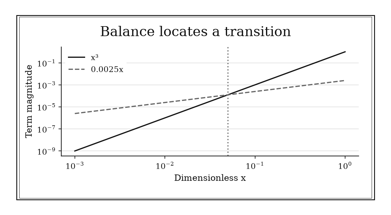
Figure 11.2. For the dimensionless constructed terms x³ and 0.0025x, equality occurs at x=0.05. Below that scale the linear term dominates; above it the cubic term dominates.
11.1.3: Express the approximation in a dimensionless small parameter
History
A thin stream of dye, injected into water flowing through a glass pipe, was the entire instrument. In 1883 in Manchester, Osborne Reynolds watched the dye stay orderly at low flow and shatter into turbulence above a threshold depending on more than speed alone: a dimensionless combination of speed, pipe size, density, and viscosity, the ratio now called the Reynolds number, built entirely from a ratio with no leftover units, so different pipes and fluids behave alike whenever it matches.
The equation
Choose a reference scale (L) and define, for example,
Then state the regime () and write an ordered expansion such as
with every term carrying the same physical units. Equivalently, scale (F) by (F_*) first and expand a dimensionless quantity.
How to read it
A dimensionless ratio is a fraction built so its units cancel, leaving a pure number meaning the same thing in millimeters or miles. A one-millimeter bump is enormous on a computer chip and irrelevant on a bridge deck; only the ratio to each scale says which. Once () is small, an approximation can be built as a base term plus corrections in powers of (), each smaller than the last, though more than one small ratio can hide a balance a single check misses.
How to use it
A pedestrian-bridge arch has a chord of 6 meters against a radius of 60 meters, and the engineer must decide whether the cheap shallow-arch formula is trustworthy, or the shop should run full circular-arc trigonometry. Forming (=L/R=6/60=0.1), the shop’s rule requires the next-order correction, (^2), to stay under 2 percent. Here (^2=0.01), 1 percent, approved; a steeper span with () gives (^2=0.25), 25 percent, and goes to full trigonometry instead.
The ratio check only covers the parameter it measures. A separate live-load deflection ratio can be numerically comparable to () without being folded in, so the engineer runs that check separately. This is a Workflow rule: it prepares a portable asymptotic calculation by making its regime and error order explicit.
11.2: Portable Large-Scale Estimates
Once the regime is clear, a small collection of estimates solves many first-pass problems. They expose factorial scale, slowly growing sums, rigorous sum bounds, geometric tails, multiplicative accumulation, and just enough remainder algebra to stop at the requested precision.
11.2.1: Use Stirling’s formula for factorial scale
History
Getting a large factorial wrong by even a small relative amount can throw off a probability calculation. In London during the 1720s and 1730s, Abraham de Moivre needed a reliable estimate of (n!) to study binomial probabilities, and derived the essential exponential shape of the factorial, though a constant remained unresolved. James Stirling supplied it, producing the familiar square-root factor built from (2): the exponential part alone does not correctly scale local probabilities, since the prefactor is smaller in order of growth, yet without it the estimate carries a stubborn error.
The equation
As (n),
Taking natural logarithms gives
How to read it
The factor ((n/e)^n) supplies the overwhelming exponential scale, the dominant term that swamps everything once (n) is large. The smaller term () is a correction riding on top: drop it and the exponential alone gets the shape right but the height wrong. Logarithms turn the product into a short sum, safer for huge (n).
The symbol () means the ratio of the true factorial to this estimate approaches one as (n) grows, a statement about the limit, not a promise the formula is exact for small (n).
How to use it
An actuary is validating a claims-simulation tool that must evaluate (n!) for batch sizes up to several hundred policies, beyond what a spreadsheet can hold as an exact integer. Checking (n=10): (), ((10/e){10}5), product (^6) against exact (10!=3{,}628{,}800); error ((3{,}628{,}800-3{,}598{,}696)/3{,}628{,}800), 0.8 percent, inside the tool’s two-percent requirement. The actuary computes the factorials in logarithmic form since raw numbers would overflow past a few hundred.
A ratio of two large batch factorials tempts a shortcut: approximating both factorials separately compounds two errors instead of one, so the actuary takes logs of the ratio and cancels shared factors first before trusting it. This is an Independent rule: it directly prices factorial-scale quantities across combinatorics, probability, statistics, and information theory.
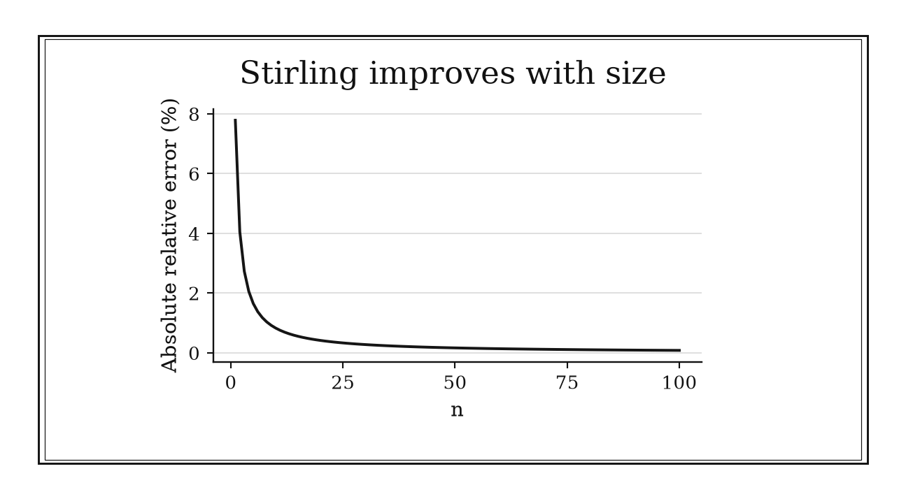
Figure 11.3. The relative error of sqrt(2pi n)(n/e)^n falls toward zero. At n=10 it is about 0.83 percent. Log-factorials avoid overflow in this comparison.
11.2.2: Estimate harmonic sums with a logarithm and Euler’s constant
History
The harmonic sum refuses to level off: added one reciprocal at a time it has no ceiling, growing forever, just so slowly that thousands of terms barely move it. From 1734 through 1740 in St Petersburg, Euler studied exactly this gap between the harmonic sum and the natural logarithm, identifying its limiting constant despite the slow convergence of the raw difference: the logarithmic integral supplies the bulk of the growth, Euler’s constant the stable leftover, an endpoint term the next correction, an estimate direct summation alone could never pin down.
The equation
The (n)th harmonic number satisfies
A common first correction is therefore
How to read it
The harmonic sum grows without bound, but at a punishing pace: multiplying the number of terms by ten only adds one copy of the natural logarithm of ten, a bit over two units. Euler’s constant, about 0.5772, is the fixed leftover once the logarithm’s growth is subtracted out, like a flat handling fee that stays the same no matter how heavy the shipment.
The extra term (1/(2n)) shrinks the remaining error; doubling (n) roughly quarters what is left, since the next piece scales like (1/n^2). The estimate assumes natural logarithms; at small (n), direct summation is safer.
How to use it
A district of 100 households needs its vaccination-outreach visits staffed; software assigns each visit slot at random among all addresses, duplicates included, until every household is reached, and the coordinator must budget the hours. The expected visit-slots needed is (100H_{100}), and (H_{100}++=4.60517+0.5772+0.005=5.18738), so the total is (100) slots, well above 100, or (519/60) staff-hours at twenty minutes each.
The estimate assumes every slot is chosen independently among all households, duplicates and all. If the software instead avoids repeating a visited address, real coverage finishes closer to 100 visits and the team is overbooked. This is an Independent rule: it directly estimates a recurring slow-growth quantity with a visible correction scale.
11.2.3: Sandwich a monotone sum with neighboring integrals
History
Bracketing a sum between two easy integrals reveals its growth rate before a single term is added up. That is what Euler’s comparison of the harmonic progression against the area under (1/x) delivered: rectangles built from (1,1/2,,1/n) sit above and below that curve, trapping the sum’s logarithmic scale immediately, well before his refined formula recovered the exact constant, a coarse first move that told Euler the answer had to grow like a logarithm.
The equation
If (f) is nonnegative and decreasing on ([1,n+1]), then
Related shifted bounds can be written for a tail beginning at another index.
How to read it
Picture the curve one-over-x with rectangles of width one stacked against it: a rectangle matching the left edge of each strip sits above the curve, one matching the right below, since one-over-x is decreasing (monotone: consistently falling, never rising). Enough strips bracket the sum between two logarithms differing by a small, fixed amount, proving growth and divergence before an exact value is found.
The bracket trades precision for certainty, and flips direction for an increasing function.
How to use it
Fifty assembly stations each need recalibration time falling off further down the line, since later stations inherit an increasingly well-tuned process: marginal time at station (k) runs about ten minutes divided by (k). Bracketing with integrals of (10/x): (10(51)(1+)), giving (39.3) minutes low and (49.1) high, so a planner schedules the window at 50 minutes without adding fifty terms by hand.
The bracket only holds if recalibration time keeps decreasing through the line. A station needing a repeat teardown near the end would leave the window short. The planner keeps ten spare minutes for that. This is an Independent rule: it directly delivers rigorous sum bounds whenever a monotone continuous comparison is available.
11.2.4: Treat a rapidly shrinking tail as its first term times a constant
History
Can a process repeated forever add up to an exact, finite number, or is trusting an endless list of ever-smaller pieces a leap of faith? Greek geometry avoided that leap. Archimedes’ Quadrature of the Parabola answered the parabola case by inscribing triangle generations in a parabolic segment in third-century BCE Syracuse, each contributing one quarter of the previous one’s area. The running total stayed bounded at every stage, proved through exhaustion to reach a limit four-thirds the first triangle’s area, trapping the true area between known figures. Every remainder was capped by a fixed multiple of the last piece counted, exactly today’s rule.
The equation
Suppose (a_k) and, for every (kn),
Then
How to read it
Suppose each new term is at most some fixed fraction, (q), of the one before, like a shrinking rebate capped at eighty percent of last month’s. The whole unseen remainder is boxed in by the first uncounted term times (1/(1-q)), near one for small (q), so that term is almost a stand-in for everything left, though as (q) creeps toward one it becomes a poor proxy for a much larger remainder.
The bound assumes the ratio holds across the tail; one that looks small early and climbs back up invalidates the certificate.
How to use it
Spoilage write-offs at a grocery chain have been shrinking each week to no more than 0.2 times the week before, thanks to a new cold-chain system, and the finance team is setting a reserve fund. This week’s write-off was ($10{,}000), so next week’s is bounded by (10{,}000=$2{,}000), and the remaining tail by (2{,}000/(1-0.2)=2{,}500) dollars, set aside instead of forecasting week by week.
If a refrigeration unit fails eight weeks out and that write-off jumps to 0.6 times the week before, the certificate breaks, so the team ties the reserve to a standing maintenance contract. This is an Independent rule: it directly converts local shrinkage into a reusable truncation certificate.
11.2.5: Take logs before estimating products
History
Multiplying and dividing long strings of numbers by hand was the daily grind of seventeenth-century astronomers, navigators, and surveyors, slow enough to limit how much work a calculator could finish in a lifetime. John Napier addressed the problem, publishing logarithms in 1614 in Edinburgh so a product could be replaced by an addition of tabulated logarithms with one lookup, the same maneuver this rule performs today: move multiplicative accumulation into additive territory, where sums are easier to control.
The equation
For positive factors (a_{n,k}),
If the log estimate is
then
How to read it
A product of many factors near one is hard to track directly. Multiply enough together and the running total can silently exceed a computer’s number format or collapse to zero. Taking the logarithm of each factor and adding instead sidesteps that, since sums behave far better than repeated multiplication near one, and exponentiating recovers the product.
An absolute error () in the summed logarithm multiplies the recovered product by (e^). Its relative error is (e^) when () is small. A small relative error in a very large log value can still mean a large absolute (), so check the log error on the scale required for the product.
How to use it
A flight-planning analyst is checking a spreadsheet that multiplies sixty sequential fuel-margin adjustments, each a factor of one plus one-sixtieth, one per route leg. Multiplying sixty numbers this close to one by hand invites rounding drift, so the analyst takes logarithms first: (P_{60}=60(1+)-), so (P_{60}e^{0.9917}), close to (e).
When the spreadsheet instead reports a combined multiplier of (3.5), the analyst knows immediately, without re-checking all sixty multiplications, that a formula is broken. The check has limits: a broken input can still leave the product near 2.7, passing the check while the formula stays wrong. This is a Workflow rule: it reorganizes a larger product estimate into a safer additive calculation.
11.2.6: Use Big-O arithmetic to keep only needed precision
History
A single capital letter, wrapped around an expression, can carry the size of an error term without its clutter of coefficients. Paul Bachmann introduced that notation in an 1894 text on number theory; Edmund Landau adopted it and developed (O), its cousin (o), and () into a toolkit in his 1909 handbook on prime distribution, letting an argument state how large a remainder was allowed to be, add and multiply those statements like algebra, and stop once smaller terms no longer mattered, though today’s compact arithmetic rules were standardized after Landau.
The equation
As (x), for (a,b>0),
and
Multiplying a bounded coefficient by (O(x^a)) preserves the same order.
How to read it
Big-O notation ((O())) is a promise about size: a quantity that is (O(x^a)) near some limit is no bigger, apart from a fixed constant, than (x^a) once close enough to that limit. Near zero, a smaller exponent means a slower-shrinking, larger quantity, so (O(x2)+O(x5)) is just (O(x^2)); multiplying two bounds adds their exponents.
These are ceiling statements: the true remainder might be smaller once cancellation is allowed for, but the bound is never exceeded, and near infinity the ranking flips: a bigger exponent means bigger.
How to use it
A calibration routine chains a lens’s forward optical transform, (1+x+O(x^2)), with its inverse, (1-x+O(x^2)), where (x) is a small alignment-offset parameter. Multiplying, the linear terms cancel: ((1+x+O(x2))(1-x+O(x2))=1-x2+O(x2)+O(x4)=1+O(x2)), so the error shrinks quadratically. Bench testing bounded the hidden constant at about 0.5, so at offset (x=0.1), the error is at most (0.5(0.1)^2=0.005), 0.5 percent, under the 1 percent tolerance, and a developer approves shipping without further correction.
The bound only says the error cannot exceed that ceiling; it says nothing about whether the true error is near it. If the hidden constant depends on a parameter the bench test did not vary, such as temperature, the measured 0.5 could understate it in deployment. This is a Workflow rule: it carries only the precision needed through a multistep expansion.
11.3: Guardrails and Escalation
Asymptotic notation is powerful because it suppresses detail. The same suppression can become dangerous under cancellation or outside a convergent series. These five rules protect ordinary calculations and identify when Euler–Maclaurin, Laplace’s method, or steepest descent is worth the extra machinery.
11.3.1: Do not subtract asymptotic equivalents blindly
History
Two quantities can grow in perfect lockstep, agreeing to every leading digit toward infinity, and still hide a finite answer after subtraction, easy to lose if trusted too far. Between 1734 and 1740, Euler ran into exactly that studying the harmonic sum and the natural logarithm: same leading growth rate, ratio tending to one, yet their difference settles on a nonzero constant, now Euler’s constant, found only by refusing to treat “grows the same way” as “negligible difference.”
The equation
If
then
but no equivalent for (f-g) follows without more terms. Write expansions through the first order that does not cancel.
How to read it
Saying two quantities are asymptotically equal only means their ratio approaches one, nothing more specific. It leaves their absolute difference open: that gap can shrink to zero, grow without bound, or settle on a fixed nonzero number, the way two staircases climbing the same steps per floor look identical from afar though the gap between them can be a constant three steps, visible up close. Subtraction is that close-up view, promoting what was too small to matter.
Rearrange first, through rationalizing or an extra expansion term, before subtracting two large, close expressions.
How to use it
A leak-detection alarm flags a pipeline segment whenever a flow-model correction drifts from expected. Write (n=Q/Q_0), where (Q) is baseline flow and (Q_0=1) cubic meter per hour; the refined and simplified models are (Q_0) and (Q_0n). A junior engineer proposes deleting the correction since their ratio approaches one and (n=1{,}000). The senior engineer rationalizes instead: (Q_0(-n)=) cubic meters per hour, essentially the half-unit buffer the alarm was calibrated around; deleting it would trigger false alarms.
The correction stabilizes near one-half only because (n) is large; for a small feeder line with (n) in single digits, the subtraction gives a different number, and the assumption needs rechecking. This is a Workflow rule: it prevents an invalid step and directs the calculation toward the first noncanceling order.
11.3.2: Stop a divergent asymptotic series near its least term
History
Add another correct term to an expansion, and the estimate can still get worse instead of better, a counterintuitive failure for anyone trained to think more terms means more accuracy. In Paris in 1886, Henri Poincaré gave a precise meaning to exactly this kind of series: it need not add to a fixed total if carried on forever, yet can approximate a function well through its first several terms even when fully divergent, its terms never tapering to nothing, explaining why an excellent early truncation can be followed by decay past its useful range.
The equation
For an asymptotic expansion
whose term magnitudes first decrease and then increase, choose a truncation index near
Under additional regularity, the best attainable remainder is often comparable to (|a_{k_*}|).
How to read it
Picture the term sizes laid out in a row: they shrink for a while, hit a smallest value, then start growing again. That smallest value is the least term, and stopping there gives an error about the size of the term itself, usually the best accuracy available, though one more term past the minimum is likely to make it worse.
This is a guide to where accuracy peaks; a certified bound needs extra analysis, and a genuinely convergent series has no reason to behave this way.
How to use it
A climate modeler is refining a temperature-projection formula by adding successive correction terms, each a smaller feedback effect. Magnitudes in degrees come out as (1, 0.1, 0.02, 0.006, 0.008,) The fourth, (0.006), is smallest; the fifth, (0.008), is larger again. The modeler stops after the (0.006)-degree term, reporting an implied uncertainty of roughly (0.006) degrees.
The modeler first confirms the series is genuinely of this divergent, eventually-growing type, since some feedback formulations in the family instead converge properly, where truncating at the same term would throw away real accuracy. This is a Workflow rule: it supplies an evidence-based stopping choice inside an asymptotic expansion rather than a standalone value.
11.3.3: Improve a sum by adding Euler-Maclaurin endpoint corrections
History
Two simple extra terms can repair a sum’s most predictable error, turning a plain integral estimate into one accurate enough to trust. Euler, in St Petersburg, and Colin Maclaurin, in Edinburgh, independently produced exactly that during the 1730s: a formula built from half the endpoint values plus a derivative correction that Euler derived in his 1735 manuscript from a Taylor expansion and tested on the harmonic sum, repairing the lattice-versus-area mismatch once the integral has captured the sum’s overall scale.
The equation
For a sufficiently smooth function,
Further Bernoulli-number terms involve higher odd derivatives, and the full theorem includes a remainder.
How to read it
An integral over a smooth curve captures the bulk of a sum’s value, the way a quick estimate of a jar of coins by its fill-level captures most of the count. Half the value at each endpoint corrects the first systematic slip, since discrete points leave a small residue at the two ends, and a further derivative term catches the curvature the integral missed.
Stacking corrections is not an invitation to add them forever: the formula can misbehave for badly chosen functions, and accuracy depends on the summand staying smooth.
How to use it
Ten zoned districts each carry an assessed value equal to the square of their district number, in thousands of dollars, and a city planner needs the total for next year’s tax projection. The integral of (x^2) from 1 to 10 is ([x^3/3]_1{10}=(103-1)/3=333). Endpoints add ((1+100)/2=50.5); the derivative correction uses the slope of (x^2), (2x), so (2=20) and (2=2), giving ((20-2)/12=1.5). Summing (333+50.5+1.5=385) thousand dollars matches the true value since higher corrections vanish for this model.
Next year’s model swaps in a formula with sharper jumps between districts, more like a step function. The correction assumes the formula stays smooth; against real jumps it will not close the gap, and the planner must split the range or use direct addition. This is a Specialized rule: it escalates from an integral estimate to a structured high-accuracy summation method.
11.3.4: Find the dominant maximum in large-parameter integrals
History
Does every part of a long integral’s range contribute meaningfully, or can almost all be ignored once a single peak dominates? Pierre-Simon Laplace answered in favor of the sliver, developing methods from 1774 into the early nineteenth century in Paris for probability integrals with a large exponential parameter: he expanded the logarithm of an integrand around its highest point, and the local, parabola-shaped approximation produced a bell-shaped estimate, the rest shrinking exponentially away, collapsing a difficult integral into a point evaluation and a square root.
The equation
Suppose () has a unique dominant interior maximum at (x_0), with
and (g) is continuous with (g(x_0)). Under standard smoothness and integrability conditions,
How to read it
Near its highest point, a smooth curve looks like a downward-opening parabola, all that matters once a large parameter multiplies the curve inside an exponential. The surviving neighborhood shrinks to a width of one over the square root of that parameter, an ordinary bell curve once rescaled.
What this does not settle is whether the maximum is really alone and interior. An edge maximum, a tie between two equally high points, or a flattened spot all break the formula.
How to use it
A sports scientist models a runner’s per-split pace deviation from goal time as (e{-nx2}), where (x) is the deviation in seconds and (n=25) measures training consistency. This needs the normalizing constant (_{-}{}e{-nx^2},dx). Matching to Laplace’s result, with ((x)=-x^2) peaking at (x=0) where (’’(0)=-2), gives (=), exact here, so at (n=25): () seconds, the peak’s effective width, and the staff sets the pacing-alert band at 0.35 seconds per split.
That width is only trustworthy because the deviation truly clusters around one peak. If the runner favors two different, equally comfortable paces, the density can develop two competing peaks, needing two centers rather than one. This is a Specialized rule: it localizes a large-parameter integral only after its dominant maximum and regularity assumptions have been verified.
11.3.5: Follow steepest descent through a complex saddle point
History
An integral that oscillates violently along its natural path can still hide a well-behaved approximation, if the path bends through the complex plane instead of the real line. That was the problem Peter Debye addressed in Munich in 1909, developing the method of steepest descent for large-order approximations to Bessel functions, used in wave and diffraction problems that resisted a good real-axis estimate, by deforming the path through a stationary point of the exponent and converting oscillation into decay.
The equation
For
find a saddle (z_0) satisfying
Locally,
Choose a path through (z_0) along which the real part of the quadratic term decreases most rapidly.
How to read it
A function’s exponent in the complex plane has both a size and a rotating phase. Along most paths that phase makes contributions cancel through oscillation, the way a shaken-up wave signal averages toward nothing. A saddle point is where the rate of change is momentarily zero, shaped like an actual saddle, rising one way and falling the other. A contour through it, where the real part falls fastest, turns oscillation into simple decay, though legality depends on singularities or branch cuts the path cannot cross.
How to use it
A phased-array antenna designer needs a fast approximation for a diffraction integral whose phase behaves locally like (iz^2) near the origin, the same shape that makes direct integration along the real axis unstable at the operating frequency. Rotating the variable, (z=e^{i/4}t), converts the exponent: (iz2=ie{i/2}t2=-t2), replacing oscillation with decay, cutting sample points by two orders of magnitude for the same accuracy.
Before trusting the result, the designer confirms no pole or branch cut sits between the real axis and the rotated path, since the material model introduces one at some frequencies, and crossing it silently would add a term never accounted for. This is a Specialized rule: it belongs to a contour-deformation workflow whose analytic prerequisites must be established before the local saddle estimate is trusted.
Chapter Synthesis , Keep the Controlling Scale
Asymptotic reasoning begins with a regime, not with deletion. Rank familiar growth classes, but locate finite crossovers when practical decisions depend on them. Balance competing mechanisms to discover where one approximation gives way to another. Express every smallness claim through a dimensionless ratio so the argument survives a change of units.
Portable estimates then compress common calculations. Stirling exposes factorial scale. A logarithm plus Euler’s constant captures harmonic growth. Neighboring integrals bracket monotone sums, while a geometric majorant certifies a shrinking tail. Logarithms turn products into sums, and Big-O arithmetic prevents irrelevant coefficients from filling the page.
The guardrails are equally important. Asymptotic equivalents cannot be subtracted blindly. A divergent expansion should stop near its least term. Euler–Maclaurin repairs a smooth sum, Laplace’s method localizes a real maximum, and steepest descent follows a legal complex path through a saddle.
Across all fourteen rules, ask four questions:
- What parameter approaches what limit, with which other quantities fixed?
- Which dimensionless ratio or balance controls the regime?
- What is the first retained term that can survive cancellation or change the decision?
- Does the rule answer the question directly, organize a workflow, or require specialized analytic machinery?
One-Page Asymptotics Toolkit
| Recognition cue | Rule to try | What it gives | Role |
|---|---|---|---|
| Familiar functions compete as (n) | Use the growth hierarchy | Eventual ranking | Independent |
| Two mechanisms exchange dominance | Equate their magnitudes | Transition scale | Independent |
| “Small” or “large” carries units | Build a dimensionless ratio | Portable regime statement | Workflow |
| A factorial is too large to form | Apply Stirling in ordinary or log form | Factorial scale | Independent |
| A reciprocal sum grows slowly | Use (n++1/(2n)) | Harmonic estimate | Independent |
| A positive summand is monotone | Compare neighboring integrals | Rigorous sum bracket | Independent |
| A positive tail shrinks by a fixed ratio | Bound by first term over (1-q) | Tail certificate | Independent |
| A product contains many factors | Take logarithms first | Additive estimate | Workflow |
| Expansions carry unused detail | Propagate Big-O orders | Precision budget | Workflow |
| Two leading equivalents are subtracted | Retain the first noncanceling order | Cancellation guardrail | Workflow |
| Asymptotic terms begin growing | Stop near the least term | Practical truncation | Workflow |
| A smooth sum needs more accuracy than its integral | Add Euler–Maclaurin corrections | Refined summation | Specialized |
| A real exponential integral has one sharp peak | Apply Laplace’s method | Local Gaussian estimate | Specialized |
| A complex phase is controlled by a saddle | Deform along steepest descent | Saddle contribution | Specialized |
Decision Path
- Is the main question about relative growth? State the limit and compare ratios. Use the hierarchy only when exponents, bases, and other parameters are fixed.
- Do two terms appear capable of competing? Equate their magnitudes, rescale at the resulting transition, and verify every omitted term afterward.
- Does “small” have physical units? Divide by a reference scale and list all independent dimensionless groups.
- Is the object a factorial, harmonic sum, monotone sum, shrinking tail, or product? Use the corresponding portable estimate before reaching for specialized machinery.
- Are expansions being combined? Decide the requested order first, then propagate Big-O remainders only to that order.
- Will leading terms cancel? Reformulate or compute another term before subtracting.
- Is a series improving and then worsening? Treat it as potentially asymptotic and compare truncations around the least term.
- Is a smooth sum or concentrated integral still too difficult? Escalate to Euler–Maclaurin, Laplace’s method, or steepest descent only after checking their specific regularity and geometry.
Transfer Problems
1. Find the regime before approximating
For
find the nonzero transition scale at which the terms are comparable. Introduce a dimensionless rescaled variable that makes both terms the same order, and state which term dominates on either side.
2. Build two different remainder certificates
First bound
from its first omitted term and a ratio. Then bracket
with neighboring integrals. Explain why the first argument gives a convergent-tail error while the second gives a growth bracket for a divergent sum.
3. Diagnose cancellation and escalation
Evaluate the limit of
without subtracting leading equivalents. Then describe the hypotheses you would check before applying Laplace’s method to an integral of the form
Where These Ideas Reappear
- Algorithms: growth hierarchies distinguish practical and eventual complexity, while crossover analysis identifies the input sizes that matter.
- Probability and statistics: Stirling, harmonic sums, Laplace localization, and Gaussian peaks control counts, tails, likelihoods, and posterior approximations.
- Differential equations: dominant balance, dimensionless ratios, boundary layers, and divergent expansions organize perturbation solutions.
- Numerical methods: Big-O arithmetic, cancellation warnings, and tail bounds become error budgets and stopping criteria.
- Information theory: logarithms convert multiplicative likelihoods into additive information, while Stirling turns multinomial counts into entropy.
- Physics and engineering: Reynolds-style scaling exposes similar systems and separates transport regimes without dependence on units.
- Complex analysis: legal contour deformation and saddle geometry determine steepest-descent approximations.
Historical Notes and Sources
All fourteen profiles have verified historical connections. The chapter distinguishes the documented mathematical or experimental act from the modern operational wording of each rule.
- Hardy and orders of growth: MAA, “Math Origins: Orders of Growth”.
- Prandtl and dominant balance: IUTAM centenary volume on Prandtl’s 1904 lecture; historical analysis of boundary-layer asymptotics.
- Reynolds and dimensionless flow regimes: bibliographic record for Reynolds’s 1883 paper; American Physical Society history of the experiment.
- De Moivre, Stirling, and factorial scale: MacTutor biography of James Stirling.
- Euler, harmonic sums, and the Euler–Maclaurin formula: English translation of Euler’s 1735 paper; Euler Archive record for E47; survey of Euler’s constant; MacTutor record of Euler’s early work on the constant; historical study of the Euler–Maclaurin formula.
- Archimedes and geometric exhaustion: translation and commentary on Quadrature of the Parabola; MAA discussion of the geometric summation.
- Napier and logarithmic calculation: Whipple Museum history of logarithmic tables; National Museums Scotland on Napier.
- Bachmann and Landau’s order notation: MAA history of order notation.
- Poincaré and divergent asymptotic series: historical study of Poincaré and divergent series; NIST DLMF, asymptotic approximations.
- Laplace’s method: historical review of Laplace’s method; NIST DLMF, Laplace’s method.
- Debye and steepest descent: Historia Mathematica history of the saddle-point method.
- Modern asymptotic statements: NIST DLMF, Chapter 2; NIST DLMF, sums and sequences.