Chapter 12: Probability: Fast Reasoning Under Uncertainty
One hundred independent components each have a failure probability of . The chance that at least one fails is not , and the linear estimate has already saturated. The exact calculation is
That quick example contains most of probability’s recurring hazards. A tiny individual risk can accumulate into a substantial system risk. Independence can make a product legitimate, but only if it is actually present. An approximation can reveal the right scale while still failing as a probability. A polished decimal is useful only after its assumptions have been named.
The thirty rules in this chapter form an uncertainty ladder. The first group starts with broad bounds and recurring scales that need little distributional detail. The second group updates beliefs and replaces exact distributions with simpler approximations, but only after earning those approximations through independence, moment, shape, or rarity conditions. The third group controls tails and audits simulation precision.
The governing habit is simple: use the weakest assumptions that answer the decision, then pay for sharper claims with stronger evidence. A bound, an approximation, and an exact probability are different products. Keeping those labels visible is more important than carrying one extra decimal place.
12.1: Bounds and Patterns That Travel
These ten rules answer common questions before a full distribution has been specified. Some give rigorous worst-case bounds; others identify collision, coverage, or rare-event scales. Their value comes from portability, and their danger comes from forgetting the conditions that make them portable.
12.1.1: Markov’s One-Moment Tail Bound
History
A single ratio, mean divided by threshold, is the entire promise behind this bound: no distribution shape required, nothing beyond the fact that the quantity cannot go negative. Working in St. Petersburg, Pafnuty Chebyshev published Des valeurs moyennes in 1867, proving that averages of many observations concentrate once variance is finite.
That paper supports the moment-bound lineage this rule descends from. Attaching Markov’s name to the compact form below is a later convention, not a claim that Chebyshev wrote this exact inequality.
The equation
If and , then
How to read it
On every outcome where reaches or passes the threshold , it contributes at least to its own average, written (its expectation, the mean value). That forces
which rearranges into the bound: a quantity that can never go negative cannot spend much probability far above a high threshold while keeping a small average.
Only one fact is spent, the mean, with no assumption about shape or spread. That is what makes the bound portable and usually loose: once exceeds one, probability’s own ceiling of one is the better number to quote.
What the bound does not tell you is how close the true chance sits to that ceiling. Equality holds only in a contrived case, so read the number as a limit on how bad things could be, not an estimate of how bad they are.
How to use it
An insurance claims analyst reviews a commercial-property line where every claim is nonnegative and last year’s book shows a mean claim of . The analyst wants a ceiling on the chance a single claim exceeds , the point where a reinsurance treaty starts paying:
The analyst books as a worst-case ceiling, not an estimate of how often the layer is hit. Claims satisfy the nonnegativity the rule needs, but the bound goes silent on a signed quantity like net underwriting profit unless applied to a transform such as . If the price hinges on whether the tail sits near or well below it, the analyst reaches for a second moment or a fitted model before signing off.
This is an Independent rule: a trustworthy mean, nonnegativity, and a threshold directly yield a portable tail certificate.
12.1.2: Chebyshev’s Distribution-Free Sigma Rule
History
A confident-looking probability can be worthless when it trusts a bell curve that was never earned. Chebyshev’s 1867 paper, the same St. Petersburg proof behind this chapter’s Markov bound, answered that risk directly: finite variance alone, with no named distribution required, was enough to cap how much probability can wander far from the mean.
The modern two-sided sigma inequality is the standard direct form of that 1867 result: refusing to assume a shape costs sharpness but buys a guarantee holding no matter what the data look like.
The equation
For a random variable with finite mean and positive finite standard deviation , and for ,
How to read it
Apply the same one-moment argument to the nonnegative squared deviation , whose average is the variance , spread measured in squared units:
Thus at least of the probability lies strictly inside a band running standard deviations, the usual yardstick for spread, either side of the mean. Distribution-free just means the guarantee holds whatever shape the data take, which is why it is weaker than a percentage built for one named curve.
At , the guarantee covers only of the probability; at it rises to . That slow, algebraic improvement is the price of refusing to assume a tail shape, not a flaw in the proof: some discrete distributions really do sit close to that or figure, so the looseness cannot be argued away.
How to use it
A supplier audit is due at a metal-stamping plant where a process engineer tracks a part dimension whose mean and standard deviation are established from gauge data, though its shape has never been confirmed as normal. Setting ,
so at least of parts fall within three standard deviations of the population mean, holding regardless of true shape. Quoting the normal-curve figure of instead would overstate the guarantee unless bell shape is independently confirmed, which it has not been. Plugging a short, drift-prone gauge run into a theorem about population moments does not deliver that same guarantee, and rare, extreme outliers do not themselves invalidate Chebyshev; an infinite or undefined variance does.
This is an Independent rule: finite population variance alone supplies a rigorous two-sided concentration statement across distributions.
12.1.3: Union Bound for Many Failure Modes
History
Ten separately unlikely failure modes stop being unlikely once the question turns to whether any one of them occurs. George Boole’s 1854 An Investigation of the Laws of Thought developed inequalities for exactly that question, bounding the chance that at least one among several events occurs; the result is still known as Boole’s inequality, or the union bound.
The modern event notation below is a direct expression of Boole’s 1854 result.
The equation
For any events ,
The useful reported bound is the smaller of the sum and .
How to read it
Write the union, the event that at least one thing happens, using flags that equal 1 when an event occurs:
Every outcome in at least one event is counted on the right at least once. Outcomes in several events are overcounted, which preserves an upper bound. No independence, no assumption that one event’s chance is unaffected by another, enters anywhere.
Strong overlap makes the result loose, but unknown dependence does not make it invalid.
Together with the obvious lower bound, it gives the quick bracket
The gap between those endpoints measures how much joint information is missing.
How to use it
Ten independent contamination checks run across a packaged-salad plant’s line, metal detection, wash-water chlorine verification, and the rest, each failing to catch a problem with probability at most . A food safety manager needs a bound before clearing the shift:
The manager books as a valid system-risk budget, valid even if some checks share a cause, such as one contaminated supplier lot. A sum exceeding one would be capped at one rather than reported as an impossible probability. Because the bound cannot say how much of that is duplicated across checks sharing a cause, checks tied to the same supplier line get a closer joint review rather than separate sign-off.
This is an Independent rule: individual event ceilings directly produce a guaranteed ceiling for their union without a dependence model.
12.1.4: Two-Term Bonferroni Correction for Overlap
History
Add up several alarm probabilities without checking whether they overlap, and the total silently double-counts every failure that two alarms share. Carlo Emilio Bonferroni, working in Florence, published Teoria statistica delle classi e calcolo delle probabilità in 1936, systematically organizing upper and lower bounds built from alternating sums of event intersections.
Retaining the individual and pairwise terms below is a direct modern use of Bonferroni’s 1936 framework.
The equation
For events ,
How to read it
The first sum counts an outcome once for every event it enters. Subtracting the pairwise intersections, the chance that two specific events both happen at once, corrects that double counting, but an outcome in three events is then subtracted too many times. The two-term expression is therefore a lower bound, not generally an exact probability.
Inclusion-exclusion alternates: odd partial sums give upper bounds, even partial sums give lower bounds.
For three events, the exact next step adds back , which is why pairwise subtraction alone undershoots whenever all three events can occur together.
If all intersections are empty, both Bonferroni endpoints collapse to the ordinary sum.
How to use it
An environmental compliance officer at a chemical plant monitors three pollutant sensors, each firing a false alarm with probability on a given shift, with each pairwise overlap between two sensors firing together at probability . Bracketing the chance that any alarm fires at all,
so the union lies in . The officer reports that range to plant management rather than either single number, and would intersect it with if an algebraic endpoint ever fell outside probability’s range. A large triple overlap, all three sensors firing during one upset, or noisy overlap estimates could leave a wide, unstable bracket, so the lower expression alone is never presented as the answer.
This is a Workflow heuristic: pairwise information tightens an earlier union-bound stage and tells you whether higher-order overlap is worth collecting.
12.1.5: Root-Sum-of-Squares for Independent Noise
History
National laboratories once combined measurement uncertainty by their own local conventions, disagreeing enough that one lab’s result could not be trusted beside another’s. In 1977 the International Committee for Weights and Measures asked BIPM to resolve the dispute; a laboratory questionnaire led to recommendations and, through an ISO working group, the 1993 Guide to the Expression of Uncertainty in Measurement, corrected and reprinted in 1995.
Root-sum-of-squares is the mathematical core of that documented consensus, with covariance restored whenever inputs share error.
The equation
For uncorrelated with variances ,
so the combined standard deviation is
How to read it
Variance is squared spread, so independent or merely uncorrelated noise powers add; standard deviations themselves do not. In the general expansion, every pair also contributes
where covariance measures whether two quantities tend to move together. Independence is sufficient for those cross terms to vanish; uncorrelatedness, a weaker condition, is sufficient for this identity.
For two unit-coefficient errors, the general standard deviation is
With , , and correlation , it is , not . Negative covariance can reduce spread, so coefficient signs and dependence direction both matter.
For uncorrelated equal-scale errors of standard deviation , the combined value is . Fully coherent errors instead add linearly, producing .
How to use it
Two uncorrelated error sources sit on a torque wrench, a sensor error with standard deviation newton-meters and a temperature-drift error with standard deviation newton-meters; a calibration technician combines them. Root-sum-of-squares gives
not the naive from adding the figures, so the wrench is certified to newton-meters combined uncertainty, with coefficients applied before squaring and units kept consistent. Shared calibration equipment or a common temperature environment can create covariance between the sources; positive covariance would make this answer understate the true uncertainty, so genuinely common systematic effects get separated out rather than labeled independent by default.
This is an Independent rule: once covariance is absent or negligible, component variances directly determine the spread of a weighted sum.
12.1.6: Total Variance: Within Plus Between
History
Every statistics course teaches that total variance splits into a within-group piece and a between-group piece; nobody can point to the paper that first proved it as a probability identity. Attribution chains reach toward analysis of variance, actuarial credibility theory, and a name sometimes attached as “Eve’s law,” but this book’s search found no secure dated event tied to this exact conditional-variance formula, so it has an evidence gap. Closing it would need a located primary paper or applied calculation that actually states the identity, dated with independent context, not a related decomposition borrowed from a nearby field. The fairest description is a standard modern identity: mathematically settled, historically unanchored.
The equation
For square-integrable and a grouping or conditioning variable ,
How to read it
Subtract and add the conditional mean, the average of within one group . The deviation of from its overall mean becomes a within-group residual plus a between-group mean shift. After squaring and conditioning on the group, the cross term vanishes because
Overall variance is therefore internal spread plus variation among group means.
Neither component can be negative, an audit: total variance must be at least each piece alone, and a violated ordering signals sampling error or a bad calculation. The identity cannot tell you whether the grouping itself is meaningful, only how variance splits once a grouping is chosen.
How to use it
A school district data analyst compares end-of-year scores across two equally sized fifth-grade classrooms. Each classroom has within-classroom variance squared points, with class means and . The mean of means is , so between-classroom variance is
Total variance is squared points, telling the analyst that classroom placement, not individual scatter, accounts for the larger share of this year’s variation. The identity is exact, but estimated components can be unstable with only two small classrooms behind them, and conditioning on a variable measured after teaching started, such as which students transferred mid-year, could produce a mathematically correct yet misleading decomposition.
This is an Independent rule: a declared conditioning structure directly partitions total variation into within- and between-group components.
12.1.7: Jensen’s Curvature Check
History
Plugging an average input into a curved cost function and calling the result the average cost quietly assumes the curve is a straight line, which most cost functions are not. Johan Ludwig Jensen, working in Copenhagen, published Sur les fonctions convexes et les inégalités entre les valeurs moyennes in 1906, centering convex functions in comparisons between a function of an average and an average of the function.
The displayed inequality is the direct modern form of Jensen’s 1906 result.
The equation
For integrable and convex on a convex domain containing both and , with well defined,
For concave , the inequality reverses.
How to read it
A convex function curves upward, like a bowl, so its graph lies below the straight line, or chord, joining any two of its points. Averaging an input before applying such a curve therefore loses the upward effect of dispersion, the spread among the values being averaged. A concave function, curving downward like a dome, gives the opposite direction.
Jensen predicts a sign, not a magnitude. Equality holds when the transformation is affine over the realized range or when the random input is effectively constant.
For a positive random variable, concavity of gives
For a two-point example with equal probability on and , while . The one-unit gap is the variance, not a numerical accident.
Both and the required expectations must exist; curvature alone cannot repair nonintegrable tails.
How to use it
A utility demand planner models the cost of meeting electricity load with a quadratic penalty, , since grid strain rises faster than load itself, forecasting mean demand megawatts with variance . Costing the mean load alone gives . But the true expected cost is
so budgeting for cost at average demand leaves grid strain running units higher than planned. The same check applies to logs, reciprocals, and growth factors, but the domain must be verified first: curvature can flip across it, and relevant expectations may not exist.
This is an Independent rule: curvature alone determines the direction of plug-in bias before a full distributional calculation.
12.1.8: At Least One Rare Event
History
A table of sparse counts, mostly zeros, occasionally a one or two, is an unlikely place to find a durable probability law. Working in Leipzig, Ladislaus von Bortkiewicz published Das Gesetz der kleinen Zahlen in 1898, analyzing deaths from horse kicks across Prussian cavalry corps-years; the sparse counts became a celebrated Poisson application.
The data and count model are historical. Interpreting the zero-count probability through today’s “at least one” shortcut is a modern extraction from that event.
The equation
For independent opportunities with common event probability ,
For rare events,
where the final step additionally requires .
How to read it
The complement, “none occur,” is a product under independence, each opportunity’s outcome unaffected by the others. Since , repeated survival becomes exponential on the exposure scale . The linear form is only the first small- expansion; unlike a probability, does not saturate at one.
For independent but unequal risks, the exact form is
Without independence, the union bound still gives , but the product and exponential approximations no longer follow. Distinguishing those statements prevents an assumption from hiding inside arithmetic.
Whenever the exact complement is cheap, use it to audit the exponential shortcut rather than replacing it automatically.
How to use it
A circuit board carries identical solder joints, each with independent failure probability over the board’s warranty life; a reliability engineer tracks them. The chance that at least one joint fails is
well below the naive linear estimate , discarded as poor once the exact complement is this cheap to compute. A shared solder-batch defect or a single reflow-oven fault would break the independence the product assumes, so the engineer checks for a common cause before trusting as the failure rate. Heterogeneous risks would instead require , and exposure units must stay consistent before is interpreted at all.
This is an Independent rule: independent repeated risks directly yield the chance of at least one occurrence and its rare-event scale.
12.1.9: Birthday Collision Threshold
History
A vast space of random identifiers is not safe simply because it is enormous: a system can start colliding identifiers long before it runs out of room. Richard von Mises, working in Istanbul, published an occupancy problem with this birthday-collision structure in 1939. Historical surveys report an earlier oral attribution, but the evidence available to this book does not settle it.
The chapter anchors the story to von Mises’s documented publication and treats the compact square-root threshold as its modern operational form.
The equation
For independent uniform draws from labels,
The collision threshold is
How to read it
There are pairs that might collide. Each pair matches with probability , so the expected collision count reaches order one when does. That is why the threshold grows like , not .
The exponential approximation uses , even though may be order one.
The halfway constant comes from setting the approximate no-collision probability to :
Replacing by then exposes the scale. The exact product remains available when that simplification is too crude.
How to use it
A uniform space of possible values holds the random 32-bit tracking IDs a backend software engineer assigns to incoming events; the engineer wants to know how many can be generated before duplicate IDs become a coin flip:
events at the halfway point, far fewer than the four billion the space suggests, a signal to widen the ID space or add a collision check well before then. Nonuniform ID generation would shorten that runway further, while dependence between draws could push it either way; near a real design boundary the exact product replaces the threshold, which is no safe operating limit.
This is an Independent rule: the size of a roughly uniform label space directly reveals the scale at which duplicates become likely.
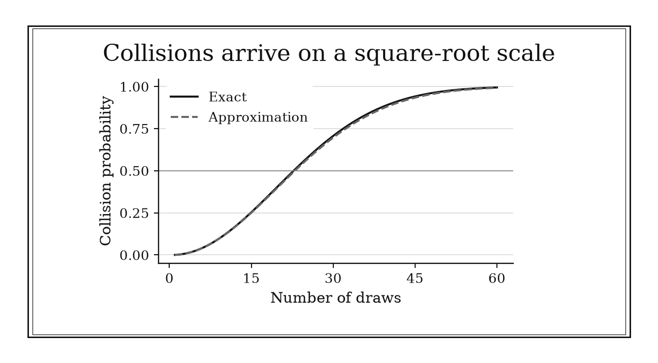
Figure 12.1. For 365 equally likely labels and independent draws, the exact collision probability passes one-half at 23 draws. This constructed uniform model excludes unequal frequencies and dependence.
12.1.10: Coupon Collector Scale
History
A collection feels nearly finished once you’ve drawn about as many times as there are categories, yet the last few categories cost far more than their share. Abraham de Moivre’s De Mensura Sortis, read to the Royal Society in London in 1711, treated waiting-time questions in games of chance. Historical studies trace the equal-probability collection problem to that work, long before commercial coupons supplied its modern name.
The harmonic formula is today’s quantitative summary of de Moivre’s question.
The equation
For equally likely categories sampled independently,
As grows,
How to read it
When categories remain unseen, the chance that the next draw is new is . The expected geometric wait for that discovery is . Summing the stages gives the harmonic factor.
The late stages dominate: finding the final category alone takes draws on average. Complete coverage therefore costs draws; alone is nowhere near enough.
The stage means are
For , the harmonic multiplier is about : repeated common categories consume most of the budget while the last unseen type remains. The mean is a long-run average, never a completion guarantee for your run.
How to use it
A warehouse operations manager is testing an automated picker against equally likely SKU bins, wanting to know how many random pick cycles are needed before every bin type has been visited at least once:
so roughly cycles is the planning mean, not a guarantee all bins are covered by then, nor a hard test deadline. The picker samples bins close to uniformly, but if one bin type is rarer in the routing logic, it could dominate the wait and blow past the planning figure. For a real pass or fail deadline, the manager calculates a completion quantile or simulates actual bin-visit frequencies instead of trusting the mean alone.
This is an Independent rule: the number of equally likely categories directly sets the expected complete-coverage scale.
12.2: Updating and Distributional Approximations
The next twelve rules exchange exactness for speed or update uncertainty with evidence. Each shortcut has an admission ticket: base rates for Bayes, a prior for succession, finite moments for the central limit theorem, recognizable distributional shape, or a rare-event regime. Check the ticket before using the approximation.
12.2.1: Bayes Updating in Odds Form
History
When nobody tracks where odds started, a rare condition can look alarmingly common the moment one positive signal comes back. Working at Bletchley Park in 1941, Alan Turing wrote about applying probability to cryptography. In Banburismus, cryptanalysts represented clues as changes in odds and as logarithmic weights of evidence, measured in bans and decibans, before spending scarce machine time.
The modern likelihood-ratio equation directly captures that Bletchley Park practice.
The equation
For complementary hypotheses and with positive prior probabilities, and evidence with ,
Posterior odds equal prior odds times the likelihood ratio.
How to read it
The prior odds carry the base rate. The likelihood ratio measures how many times more compatible the evidence is with one hypothesis than the other. Evidence multiplies existing odds; it does not erase where the update began.
Taking logarithms makes successive conditionally independent likelihood ratios additive, meaning each new piece of evidence adds no leftover information about the others once the hypothesis is fixed. Without that conditional independence, multiplying marginal ratios can count the same information twice.
Probability converts to odds , and odds convert back to . A likelihood ratio of one leaves odds unchanged; values above one favor , and values below one favor . Direction and base rate are therefore visible before conversion back to probability.
How to use it
A condition has prevalence in a patient population, giving prior odds ; a hospital diagnostician is evaluating a screening test for it. A positive result carries a published likelihood ratio of , updating the odds to :
That is neither the the raw ratio suggests nor near certainty, so the diagnostician orders a confirmatory test rather than acting on alone, first checking that the test’s published performance came from a population like this one and that any second signal stays independent of the first once conditioned on each hypothesis.
This is an Independent rule: prior odds and a defensible likelihood ratio directly produce updated odds across binary evidence problems.
12.2.2: Laplace Rule of Succession
History
Few results in probability have been argued over as long as Laplace’s sunrise calculation, and the argument began with Laplace himself. Working in Paris, he gave a predictive probability after repeated successes in his 1814 Essai philosophique sur les probabilités, then immediately warned that the famous stylized sunrise version of it ignored relevant physical knowledge.
Both the rule and the caveat are documented: a mathematical update is only as appropriate as the exchangeability model and prior behind it.
The equation
With successes in Bernoulli trials and a prior,
and the posterior mean, also the next-trial predictive probability, is
How to read it
The uniform beta prior contributes one notional success and one notional failure. This prevents a short perfect record from becoming a probability of exactly one and prevents zero observed successes from becoming permanent impossibility.
The pseudo-counts are a prior choice, not objective data. Other knowledge should produce other prior parameters.
Observed failures equal , so the posterior has parameters and . Before any observations, its mean is ; as grows, the two prior counts become less influential. This makes the amount of smoothing explicit.
How to use it
A supplier quality manager reviews a new parts supplier’s qualification run of ten units, all ten passing inspection. Rather than reporting a raw pass rate, the manager applies the smoothed estimate:
That leaves room for a future defect while still crediting the clean run, and the manager uses it to set a conservative reorder quantity rather than treating the supplier as flawless. The shortcut only holds if the ten units can reasonably share one constant defect probability and were tested independently; a known process change partway through the run would break that assumption, and no stylized prior should override solid physical knowledge about how the parts were made.
This is an Independent rule: under an explicit uniform beta prior, a success count directly yields a smoothed predictive probability.
12.2.3: Central-Limit Approximation for a Sample Mean
History
Why does averaging many small, unrelated measurements settle into the same bell-shaped pattern almost every time, whatever the individual measurements look like? Working in London, Abraham de Moivre circulated his Approximatio ad Summam Terminorum Binomii in 1733, replacing a large symmetric binomial sum with a bell-shaped integral and calculating its tail areas. His theorem concerned that one symmetric binomial problem, not arbitrary sample means.
The general sample-mean central limit theorem is a later extension of that 1733 normal-approximation breakthrough.
The equation
For iid observations with mean and positive finite variance ,
as .
How to read it
Centering removes the population mean, and multiplying by offsets the shrinking spread of an average. Under the stated conditions, the standardized distribution approaches a universal normal shape.
The arrow is a limit, not a finite-sample error guarantee. Convergence speed depends on skewness, tails, dependence between observations, and whether a central or an extreme probability is being approximated.
Independence, each observation carrying no information about the others, also gives
That identity explains the standard-error scale even before normality is invoked. Quadrupling halves the spread, while the CLT separately supplies the approximate shape used for probability calculations.
How to use it
An agronomist samples yield from independently managed test plots of a new wheat variety, mean bushels per acre, standard deviation bushels. The sample mean has
bushels, so central sampling probabilities for the trial average approximate , but only after checking plot yields are roughly independent and not dominated by a few outlier fields. There is no universal “” permission slip: a drought-damaged corner, or irrigation shared across nearby plots, would break independence and demand more plots before the approximation is trusted.
This is an Independent rule: suitable repeated sampling directly supplies the normal scale and spread of a sample mean.
12.2.4: The 68-95-99.7 Normal Rule
History
Three memorized percentages, , , and , are the entire artifact behind this rule: a portable digest of a tail-area calculation nobody needs to redo by hand. De Moivre’s 1733 binomial approximation, the same bell-shaped curve behind this chapter’s central-limit rule, supplied the early version of that calculation. The three figures are a modern teaching digest, not wording from his pamphlet.
The mnemonic remains explicitly conditional on normal shape.
The equation
For ,
How to read it
Standardization turns any normal variable into . The three numbers are areas under the standard normal curve between symmetric cutoffs.
They describe a distribution, not every dataset that has a mean and standard deviation. Compare with Chebyshev’s much weaker but distribution-free guarantee.
By symmetry, the mass outside is about , split roughly into each tail. Outside it is about total. Those complements are often more useful for alarms than the inside percentages.
These figures use population and ; estimating them from the same small sample adds uncertainty.
How to use it
A packaging quality auditor at a snack-food plant reviews independent bag weights from a filling line that has run stable and nearly normal for months. The mnemonic predicts bags within of target weight and bags beyond per batch, expectations the auditor uses to set a routine reject-rate alarm, not fixed quotas to hit exactly. Before trusting the numbers, the auditor checks a histogram of recent weights: a sticking filler valve or a heavy right tail from occasional overfills would create far more extremes than the rule predicts. When a customer complaint hinges on the gap between “about ” and a calibrated probability, the auditor runs exact normal software instead of the mnemonic.
This is an Independent rule: once a normal model is justified, standard-deviation distance directly translates into memorable probability mass.
12.2.5: Normal Approximation to a Binomial Count
History
Treated as safely bell-shaped without a second thought, a binomial count can betray that assumption exactly where it sits near zero or near its ceiling, right when a decision depends on it. De Moivre’s 1733 work, met once already in this chapter, matched a bell curve to those binomial counts and read their tail areas directly; later work generalized his symmetric case to any success probability.
The normal approximation descends directly from that calculation. The familiar “expected successes and failures near ten” screen is a modern guardrail, not de Moivre’s own constant.
The equation
For , use
when both
How to read it
A binomial count is a sum of independent Bernoulli variables, each a coin-flip-like trial. The two checks keep both expected successes and failures away from zero, screening out severe skew, a lopsided distribution with one tail longer than the other, and a nearby boundary.
The normal is continuous while the binomial is discrete. A half-unit continuity correction usually improves moderate-sample probability calculations.
The binomial skewness is
The success–failure checks make its magnitude smaller and keep the normal curve from assigning substantial area beyond or . They are screening rules, not a uniform accuracy guarantee.
How to use it
A clinical trial statistician expects enrolled patients to respond to a treatment at rate , based on prior trials. The normal approximation gives
so counts from about to span roughly two approximating standard deviations, the range the statistician uses to flag whether an interim count looks unusually low or high. Near the trial’s stopping boundary, the statistician switches to exact binomial calculations rather than trusting the approximation, and watches for site-to-site heterogeneity in response rates, which can inflate variance beyond what this formula assumes. For a cumulative event such as , standardizing using mean and standard deviation keeps the correction explicit and reproducible.
This is a Workflow heuristic: it selects a faster continuous approximation after the binomial structure and success–failure conditions have been checked.
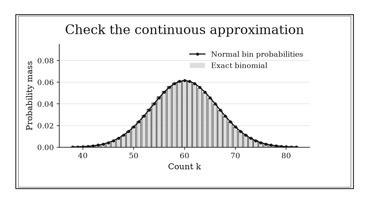
Figure 12.2. For Bin(200,0.30), normal probability over each half-unit bin closely tracks the exact mass near the center. Tail decisions still warrant exact calculation; the success-failure checks are only a screen.
12.2.6: Normal Approximation to a Poisson Count
History
Two famous nineteenth-century results sit on either side of this rule, Poisson’s rare-event counting and de Moivre’s bell-shaped binomial approximation, yet no located paper welds them into this specific Poisson-to-normal shortcut. Combining the two into one invented episode would manufacture an event neither mathematician recorded, so the rule has an evidence gap: the search verified Poisson’s 1837 Recherches and de Moivre’s 1733 work, but found no dated event for this exact approximation or its modern -near-ten threshold. Closing the gap would need a primary source that states or applies the joint rule, not two ingredients standing near each other in a textbook. The chapter presents it as contemporary practice instead.
The equation
If , approximate
commonly screening for
How to read it
A Poisson count has mean and variance both equal to , standard deviation , and skewness, a lopsidedness with one tail longer than the other, equal to . As grows, relative skew falls and the central part becomes more bell-shaped.
The threshold is a heuristic, not a theorem guaranteeing a requested error. Lower tails remain constrained by zero, and far-tail relative errors can be poor.
Relative standard deviation is
At it is , and skewness is also . Increasing reduces both, explaining the direction of improvement without certifying the cutoff.
The screen is intended for central probabilities; a large mean alone does not guarantee accurate extreme tails.
How to use it
An emergency department charge nurse tracks overnight patient arrivals, historically averaging per shift, so the standard deviation is . Two standard deviations bracket the range to arrivals, with a half-unit correction for a specific integer count, flagging an unusually heavy or light shift for staffing. For a rare quiet night near zero, or a staffing call that hinges on the exact tail, the nurse calculates the Poisson probability directly. If arrival counts run more variable than the mean suggests, perhaps from clustered ambulance runs after a highway incident, that overdispersion signals a different count model is needed.
This is a Workflow heuristic: it routes a verified Poisson model to a normal calculation only after scale and tail location are judged adequate.
12.2.7: Half-Unit Continuity Correction
History
A discrete count meeting a continuous curve without its half-unit adjustment leaves a probability estimate quietly shifted by a small systematic sliver. De Moivre’s 1733 work, the refinement layer on the bell-curve approximation used elsewhere in this chapter, replaced a sum of discrete binomial masses with continuous area; placing an integer mass inside a unit-width cell is the modern geometric refinement of that calculation.
The half-unit convention lines the area up with whole probability bars rather than their centers.
The equation
For an integer-valued approximated by continuous ,
More generally, maps to .
How to read it
The mass at integer corresponds geometrically to the continuous cell . Shifting an endpoint captures the complete boundary cell instead of cutting through its center.
For a continuous , strict and non-strict inequalities have the same probability, but the integer event must be translated carefully.
The correction is easiest to audit by drawing unit cells centered at the included integers: an event containing one endpoint but not the next ends halfway between their centers, which prevents memorized “plus or minus ” rules from reversing a tail. The half-unit shift cannot repair skew or a wrong model.
How to use it
A plant quality control lead approximating the count of defective units on a shift, defects, with a matching normal distribution standardizes , not . For , the integer values covered are through , so the lead uses continuous limits and . The correction reduces discretization error only, so the lead writes down the original integer event before moving either boundary; it will not rescue a batch-dependent or genuinely skewed count.
This is a Workflow heuristic: it refines a discrete-to-continuous approximation after the normal route has already been selected.
12.2.8: Berry-Esseen Check on CLT Accuracy
History
The probability estimate that follows a central-limit claim can carry an error nobody has actually bounded. Andrew Berry’s 1941 paper bounded exactly that distance, between a standardized sum and the normal curve; Carl-Gustav Esseen independently sharpened and systematized the analysis in work culminating in 1945.
Their documented achievement gave the central limit theorem a finite-sample rate. The universal numerical constant has been improved since their papers.
The equation
For iid with mean , variance , and , let . Then
with a universal .
How to read it
The standardized third absolute moment prices tail weight and asymmetry, while gives the worst-case rate. The bound controls the absolute error in the cumulative probability curve (CDF) uniformly in .
Uniform absolute error can still be useless for a tiny tail: an error ceiling of does not validate a probability near .
The bound scales linearly with the standardized third absolute moment. Doubling that ratio doubles the certificate; quadrupling halves it. Those relationships turn Berry–Esseen into a sample-size and tail-shape diagnostic even when its numerical ceiling is conservative.
How to use it
A portfolio risk analyst considers a model of iid daily returns with finite third absolute moment and an established population bound . To audit a normal approximation for the standardized sum, the analyst calculates
so the analyst treats the approximation’s CDF error as at most percentage points, rigorous but possibly loose, before relying on it for a routine risk report. An empirical moment ratio estimated from those same 400 days would be only a diagnostic, not this population guarantee. The analyst must justify the iid model and the moment bound; for the extreme tail behind a stress-test capital requirement, sharper distribution-specific analysis replaces this bound entirely.
This is a Workflow heuristic: it audits whether a proposed CLT approximation has a defensible finite-sample error scale.
12.2.9: Poisson Approximation to a Binomial Count
History
This section already earned a bell curve for binomial counts once both successes and failures pile up by the dozens; the opposite regime, where successes stay rare no matter how many trials run, is what Siméon-Denis Poisson worked out in Paris, publishing Recherches sur la probabilité des jugements in 1837. Beyond its framing around whether juries reach correct verdicts, the treatise developed probability approximations for many Bernoulli opportunities with small individual probabilities.
The rare-event limit is the historical anchor; today’s numerical screening rules were attached later.
The equation
For , set and use
when is large and is small.
How to read it
As grows and shrinks with held fixed, the binomial mass converges to the Poisson mass. Individual opportunity details collapse into the expected count .
This approximation is built for rare events; large alone does not justify it. A large retains binomial asymmetry and finite-capacity effects.
The limiting calculation preserves the expected count because both models have mean . Their variances differ:
Small makes that discrepancy small and shows why the approximation worsens as grows.
How to use it
An extension agronomist samples plants for a pest that infests each independently with probability , so . The approximation gives
close to the exact binomial value near , and the agronomist uses that to judge whether an infested-plant count of or fewer is unremarkable before recommending treatment. Were the infestation rate closer to one, the agronomist would count the rarer healthy plants instead. Clustered infestation can break independence; different plant-level rates can preserve independence but break the common-probability binomial model. The agronomist uses a model matching that structure and an exact calculation whenever the decision is close.
As a quick internal check, the Poisson point mass at three is . Summing point masses must stay between zero and one and approach one as the upper limit grows.
This is a Workflow heuristic: it replaces a verified rare binomial count with a simpler Poisson calculation inside a larger probability workflow.
12.2.10: Exponential Approximation to a Geometric Wait
History
Waiting for a rare discrete event step by step turns awkward once the steps are many and each one’s chance is tiny; a continuous stand-in removes the awkwardness. Bortkiewicz’s 1898 horse-kick study, already put to work earlier in this chapter, documented a Poisson application: a Poisson process has exponential waiting times, while Bernoulli trials instead have geometric waits.
Using that connection for the small- scaling below is a modern process interpretation; the historical book did not derive or name this approximation.
The equation
Let count trials through the first success, with success probability . For integers ,
so as ,
How to read it
The approximation follows from . When each step carries a tiny hazard, discrete survival over steps resembles continuous exponential survival over scaled time .
Stating the geometric convention matters: some definitions count failures before success and begin at zero.
Under the convention used here,
matching the mean of . If a convention uses failures before success, it replaces by ; after multiplication by small , that one-step difference vanishes asymptotically but not in an exact short wait.
The exponential surrogate also puts the median wait near , since at that point. This is shorter than the mean , reflecting the long right tail.
How to use it
A site reliability engineer models a service crashing on any given deploy with probability per deploy, and wants the chance the service survives past deploys without a crash:
The approximation is excellent at this scale, so the engineer plans capacity using the exponential surrogate rather than tracking each deploy. If is not small but remains constant across independent releases, return to the exact geometric calculation. For independent releases with varying crash probabilities , survival through releases is instead; clustered crashes require a model of their dependence.
This is a Workflow heuristic: it selects a continuous waiting-time surrogate after a rare, constant-probability discrete process has been established.
12.2.11: Lognormal Mean Correction
History
Two different numbers can each honestly claim to be the “typical” value of the same skewed measurement, and the gap between them is structural, not an error. Working in London, Donald McAlister described that structure in an 1879 paper on a skewed “law of frequency” arising from multiplicative rather than additive effects; the paper is recognized as an early derivation of the distribution later called lognormal, distinguishing its geometric center from its arithmetic mean.
The compact correction below is the modern parameterization of McAlister’s distinction.
The equation
If
then
How to read it
Exponentiating the mean log returns the median because . The arithmetic mean is higher by the factor because the convex exponential transformation gives extra weight to the right tail.
The variance here is log-scale variance, not variance of in original units.
The mean-to-median ratio is
It grows with log-scale dispersion and is another exact illustration of Jensen’s inequality for the convex exponential function. Zero variance makes the two summaries coincide.
The formula uses the natural logarithm. Another log base requires conversion before applying the exponential correction.
How to use it
An environmental scientist models groundwater contaminant concentration, in micrograms per liter, as lognormal, with log mean and log variance estimated from monitoring wells:
Reporting only as “the mean” concentration to a regulator would understate the true arithmetic average by nearly a full microgram, since the exact correction factor requires normal log errors and the log-scale variance used here. If different wells show different scatter around their own logs, that heteroskedasticity calls for an observation-specific correction or a smearing estimate rather than one global factor.
This is an Independent rule: a normal log model directly determines the distinction between median and arithmetic mean on the original scale.
12.2.12: Delta Method for a Smooth Transformation
History
A technique used constantly in applied statistics, rescaling a standard error through a smooth function’s derivative, carries a name, “the delta method,” that nobody can trace to a founding paper. Retrospective accounts reach toward early error propagation, Taylor approximations, and general asymptotic theory, and one 1981 paper on standard errors gets mentioned often, but this book’s survey found no securely dated discovery or real application of this exact rule, so it has an evidence gap. Closing it would need a primary source that actually states and applies the transformation rule, not a later paper merely discussing standard errors nearby. The mathematics is well supported; the chapter presents it as established technique rather than inventing an origin.
The equation
If
and is differentiable near with , then
How to read it
A first-order Taylor expansion, approximating a smooth function by its local slope, gives
The transform therefore multiplies standard error by , the size of that slope. The method is local and asymptotic; curvature and boundary effects are omitted at first order.
The variance rule is
Because the derivative is evaluated at an unknown parameter, applications usually plug in . That extra approximation is harmless only when the derivative changes little over the estimator’s uncertainty range.
How to use it
An economist estimates a regional price index at with standard error , and needs the uncertainty of its log for a growth-rate model, :
The economist reports that log-scale standard error, trusting the plug-in derivative because the estimate sits well inside a smooth neighborhood, far from zero. A nonsmooth transform, a ratio with a near-zero denominator, or a point where would call for higher-order treatment; transforming a confidence interval endpoint-by-endpoint is the safer fallback when monotonicity is available.
This is a Workflow heuristic: it propagates an existing asymptotic uncertainty calculation through a smooth transformation rather than standing alone.
12.3: Tail Control and Simulation Diagnostics
The final eight rules ask what extra information buys beyond moment-only bounds. Direction, boundedness, variance, sub-Gaussian decay, and a known normal tail each sharpen risk control differently. The section then turns to simulations, where nominal draw count can conceal slow root- precision or severe weight degeneracy.
12.3.1: Cantelli’s One-Sided Variance Bound
History
Paying for two-sided protection when only one direction of risk actually threatens a system wastes exactly the safety margin that matters. Francesco Paolo Cantelli’s 1928 Italian publication Sui confini della probabilità included the one-sided probability inequality now bearing his name, directing mean-and-variance information toward one tail instead of paying for both.
The directional-risk interpretation below is a direct modern reading of Cantelli’s 1928 result.
The equation
For a random variable with finite mean , finite variance , and ,
When , setting gives .
How to read it
Chebyshev bounds the combined event that either tail exceeds a distance. Cantelli uses a shifted squared-moment argument to keep the direction, producing a slightly smaller ceiling for one-sided risk.
The inequality still knows nothing about skewness or tail shape. It is a rigorous worst-case statement, not an estimate of how the present distribution usually behaves.
The corresponding lower-tail statement follows by applying the rule to :
Choose one direction before calculating; adding the two one-sided ceilings recreates a valid but usually inferior two-sided statement.
How to use it
A grid operations analyst worried only about overload, not shortage, bounds the chance that load reaches three standard deviations above the historical mean:
Two-sided Chebyshev would give the looser after discarding lower-tail coverage the analyst never needed. Cantelli fits because only one direction, overload, threatens the grid, and the population moments are credible; estimated moments carry uncertainty the formula doesn’t show, so the true overload chance could sit well below this bound.
This is a Workflow heuristic: it selects the one-sided member of the moment-bound toolkit after the risk direction has been identified.
12.3.2: Hoeffding Bound for a Bounded Sample Mean
History
Wait for a sample to grow large enough for the central limit theorem to apply, and a decision that cannot wait is left with no finite-sample guarantee at all. Working in Chapel Hill, Wassily Hoeffding published a systematic family of probability inequalities for sums of bounded independent variables in 1963, supplying exponential guarantees without specifying a full distribution.
The sample-mean formula is a direct specialization of Hoeffding’s 1963 paper.
The equation
If independent with , then for ,
Cap the right side at when necessary.
How to read it
Independence makes exponential moments multiply, while the hard range limits how large each factor can become. The result shrinks exponentially in and does not need a variance estimate or identical distributions.
That robustness costs tightness: observations concentrated in a small part of the allowed range may concentrate much faster.
The inequality can also be inverted. To make the failure probability at most , it is sufficient that
This turns a tail theorem into a conservative sample-size plan.
How to use it
An education researcher scores independent student assessments on a scale and wants a guarantee on the sample mean within of the true average score:
The researcher trusts this only because the range is genuinely honest and every assessment is independent; students sharing one teacher effect, or scores collected only from those who finished early, would invalidate the basic form. If the true score variance is known to be much smaller than the range suggests, Bernstein’s bound gives a tighter guarantee instead.
This is an Independent rule: independence, a hard interval, and sample size directly supply a nonasymptotic mean-error guarantee.
12.3.3: Multiplicative Chernoff Bound for Counts
History
When only an expected count gets reported, without asking how far short a real count could plausibly fall, a system failure can hide as ordinary noise until it’s too late. Herman Chernoff, working at Stanford in 1951 and 1952, developed exponential-moment bounds while studying the efficiency of hypothesis tests based on sums of observations.
The optimization principle is historical. The compact multiplicative formulas for independent Bernoulli counts are standard modern descendants of that documented method.
The equation
For a sum of independent Bernoulli variables with and ,
For ,
How to read it
Exponentiating a sum turns it into a product. Markov’s inequality bounds the exponential tail event, and optimizing the exponent produces a decay rate tuned to the requested relative deviation.
Unlike an additive bound, the scale is the expected count . A -count shortfall means something different when than when .
The exponent grows linearly with for a fixed relative deviation, so doubling the expected count squares a bound of the form : multiplicative concentration becomes powerful for large, stable counts. The bound is a ceiling, never an estimate; near the mean it is wildly conservative.
How to use it
A data center capacity planner expects successful health-check pings per hour across a server fleet; observing or fewer corresponds to :
The planner treats a drop to as strong evidence against the healthy independent-ping model, given this small upper bound, and investigates an outage or another model failure. The bound alone does not give the probability that an outage occurred; that would also require an outage prior and an alternative model. Dependence between pings is one possible reason the healthy model could fail.
This is an Independent rule: the expected count and a relative deviation directly yield an exponential tail certificate under Bernoulli independence.
12.3.4: Bernstein’s Variance-Aware Tail Bound
History
Choosing between a variance-based bound and a range-based bound turns out to be a false choice: the sharpest guarantee uses both, trading one for the other as the deviation grows. Sergei Bernstein’s 1920s Soviet work struck exactly that compromise, strengthening moment-based bounds with exponential tails for sums of independent variables.
The constants vary among formulations; the equation below is the standard modern bounded-sum form supported by that history.
The equation
If independent variables satisfy, for some ,
almost surely, let
Then, for ,
How to read it
When is moderate, dominates the denominator and the exponent looks Gaussian, proportional to . For very large , the term prevents a falsely optimistic Gaussian tail.
Bernstein can improve on a range-only Hoeffding bound when actual total variance is small, but it needs that variance information.
The crossover is visible in the denominator. When , the variance term dominates; when , the range term dominates. A two-sided version can be obtained by applying the bound to both the sum and its negative and adding the two tail ceilings.
How to use it
Many independent route legs each contribute delivery-time deviations bounded by hour from their own mean, with total variance across the legs; a logistics network planner sums the centered deviations and wants the chance the network-wide deviation reaches hours:
a tight guarantee the planner trusts only after checking the legs are genuinely independent and that is a real almost-sure bound rather than the worst leg observed so far. Plugging in a sample variance instead of the population value would need an empirical-Bernstein correction not applied here.
This is a Workflow heuristic: it selects a variance-sensitive concentration bound after boundedness and variance information have been verified.
12.3.5: Maximum of Many Sub-Gaussian Errors
History
Why does the largest of many independent measurements grow so slowly as more are added, rather than growing in proportion to how many there are? R. A. Fisher and L. H. C. Tippett’s 1928 Cambridge paper founded limiting theory for sample maxima, explicitly studying normal samples and showing that extremes live on a different scale from typical observations.
The sub-Gaussian threshold is a modern concentration summary of that 1928 extreme-value phenomenon.
The equation
For and , if every satisfies, for , the one-sided tail bound
then
Setting the right side near one suggests
How to read it
The union bound alone proves the upper probability inequality, so it does not require independence. The square-root-log scale follows by balancing one light tail against opportunities.
Independence matters when treating this upper scale as typical. Strong positive dependence can make the effective number of distinct opportunities much smaller, while heavy tails change the scale entirely.
For a desired familywise ceiling , solve the union bound for
Then . This adds the confidence requirement that the order-one scale deliberately omits.
How to use it
A research lab running parallel assay channels, each with unit-scale normal noise, expects its largest fluctuation near
standard deviations by chance alone, not evidence of a real effect. This first-order scale isn’t a calibrated extreme quantile, so the lab still checks channel dependence, tail shape, and whether the flagged channel was chosen only after looking at the data.
This is an Independent rule: a sub-Gaussian marginal tail and the number of comparisons directly set a portable maximum-error scale.
12.3.6: Mills-Ratio Approximation for a Normal Tail
History
Printed normal tables stopped short exactly where a calculation needed the deep tail. John P. Mills tabulated a ratio of tail area to curve height at the cutoff in a 1926 paper, giving small normal-tail calculations a fast, hand-computable shortcut.
The approximation and bracket below are direct modern forms of Mills’s 1926 quantity, valuable when tables or digital computation are unavailable.
The equation
For , with standard normal density and CDF ,
The rigorous bracket is
How to read it
The normal density falls so quickly that the area beyond is governed largely by its boundary height. Integration by parts shows that the local logarithmic slope supplies the dividing scale.
The upper approximation becomes relatively accurate far into the tail. Near zero, division by makes it useless.
At , the bracket itself gives
or approximately . The exact tail sits close to the lower endpoint, illustrating both the guarantee and the approximation’s direction.
For mental use, wait until is at least roughly two; near the center, use normal tables or software.
How to use it
A floodplain engineer checking the chance rainfall exceeds three standard deviations above normal, , gets
close to the exact one-sided tail of about , good enough for a quick design check before running the full survival-function routine used for the final report. But rainfall tails are rarely this tidy: a skewed, non-normal tail can make overstate or understate the true exceedance, so the engineer cross-checks the empirical tail before filing.
This is an Independent rule: a positive normal score directly yields a fast tail approximation and rigorous elementary bracket.
12.3.7: Monte Carlo Error Falls as One Over Root N
History
Doubling a simulation’s sample size feels like real progress until the error barely moves, and a budget planned around that mistaken intuition runs out fast. Nicholas Metropolis and Stanislaw Ulam, working at Los Alamos, published The Monte Carlo Method in 1949, describing repeated random sampling made practical by electronic computation.
The root- precision law is the modern sampling-theory account of the computational method established by that paper.
The equation
For iid draws and an integrand with finite variance ,
How to read it
Independent variances add across the sum, while dividing by squares in the variance. The resulting variance becomes standard error.
Halving random error needs four times as many draws. Gaining one decimal digit, tenfold smaller error, needs roughly one hundred times as many.
In practice is unknown and is replaced by the sample standard deviation of . That estimates random sampling error only. It does not reveal deterministic coding error, discretization bias, burn-in bias, or a target distribution implemented incorrectly.
Solving the rule for a target standard error gives the planning equation . A pilot run can estimate , after which the budget should be updated rather than guessed.
How to use it
A grid planning team simulating outage risk finds that draws give standard error ; reaching for a regulatory filing requires approximately
draws, a hundredfold increase the team budgets compute time for rather than assuming a modest rerun will do. The team estimates from the pilot run and reports Monte Carlo uncertainty alongside the answer, aware that serial correlation between draws would replace nominal with a smaller effective sample size.
This is an Independent rule: finite-variance independent sampling directly prices the simulation budget needed for a target random error.
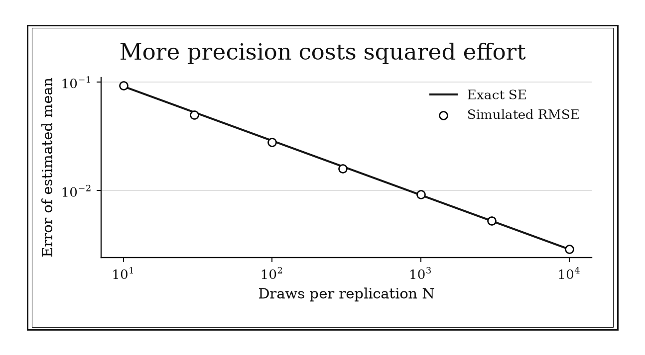
Figure 12.3. For iid Uniform(0,1) draws, the mean has exact standard error sqrt(1/(12N)). The simulated RMSE across 400 independent replications follows that scale with finite-replication noise.
12.3.8: Importance-Weight Effective Sample Size
History
Ten thousand simulation draws can flatter a result that a handful of dominant weights actually produced. Augustine Kong, Jun Liu, and Wing Hung Wong published a sequential-imputation method for Bayesian missing-data problems in 1994, interpreting importance-weight variability through an effective sample size.
The widely used inverse-squared-weight formula comes straight from that 1994 diagnostic; treating it as a universal variance equivalence goes beyond it.
The equation
For proposal draws , let
The diagnostic is
How to read it
Uniform normalized weights give ; one dominant weight drives it toward one. The formula measures realized weight concentration and quickly exposes a proposal that sends most computation to nearly irrelevant draws.
It ignores how the integrand aligns with those weights and cannot reveal target regions that the proposal never visited.
Because normalized weights sum to one,
Multiplying all raw weights by the same positive constant leaves the diagnostic unchanged. These properties make it an easy implementation check, but not a proof of accurate integration.
How to use it
A data science team running an importance-sampling simulation with draws finds one normalized weight at and the other each at :
meaning nearly all nominal draws contribute almost nothing, so the team inspects the maximum weight, replicate estimates, and proposal support before trusting the result. Heavy-tailed weight ratios can make the diagnostic itself unstable.
This is a Workflow heuristic: it audits an importance-sampling stage and decides whether proposal repair or resampling must follow.
Chapter Synthesis: Climb the Uncertainty Ladder Deliberately
Probability shortcuts become reliable when their information requirements are visible.
Start with the weakest defensible statement. Markov needs nonnegativity and a mean. Chebyshev and Cantelli spend a variance. The union bound needs only marginal event probabilities, while Bonferroni spends intersection information. These are guarantees, often conservative, and should be labeled as bounds rather than predictions.
Next recognize scale. Independent noise combines through squared standard deviations. Rare repeated risks accumulate through , collisions emerge near , and complete coverage costs . These patterns travel widely because they describe structure rather than one named dataset.
Earn approximations through assumptions. Bayes requires a base rate and likelihood model. Normal, Poisson, exponential, lognormal, and delta approximations require their own shape, rarity, smoothness, or moment conditions. Continuity correction improves a viable approximation; it cannot rescue a bad one. Berry–Esseen asks how much finite-sample confidence the central limit theorem has actually earned.
Finally audit tail and simulation claims. Boundedness, variance, and sub-Gaussian decay buy progressively sharper concentration. Monte Carlo still pays the tax, while importance weights can reduce thousands of nominal samples to only a handful of effective contributors.
Across all thirty rules, ask:
- Is this number exact, an approximation, or a bound?
- Which assumption, independence, finite moments, boundedness, normality, rarity, or smoothness, licenses it?
- Is the rule answering the question or checking one stage of a larger workflow?
- Would dependence, heterogeneity, tail shape, or model drift reverse the decision?
One-Page Probability Toolkit
| Recognition cue | Rule to try | What it gives | Role |
|---|---|---|---|
| Nonnegative quantity, only its mean known | Markov | One-moment tail ceiling | Independent |
| Mean and finite variance, unknown shape | Chebyshev | Two-sided sigma guarantee | Independent |
| Any of many events may occur | Union bound | Dependence-free union ceiling | Independent |
| Pairwise event intersections known | Two-term Bonferroni | Lower–upper union bracket | Workflow |
| Uncorrelated error contributions | Root-sum-of-squares | Combined standard deviation | Independent |
| Mixture or grouped population | Total variance | Within-plus-between split | Independent |
| Nonlinear transform of random input | Jensen | Direction of plug-in bias | Independent |
| Many independent rare opportunities | At least one | Exact complement and Poisson scale | Independent |
| Duplicate risk in labels | Birthday threshold | Collision scale | Independent |
| Need every one of labels | Coupon collector | Coverage scale | Independent |
| Binary evidence update | Bayes in odds form | Posterior odds | Independent |
| Short Bernoulli record | Laplace succession | Smoothed predictive probability | Independent |
| Average of many iid observations | Sample-mean CLT | Approximate normal sampling law | Independent |
| Distribution is credibly normal | 68-95-99.7 rule | Quick sigma frequencies | Independent |
| Binomial center with both counts large | Normal approximation | Faster count probabilities | Workflow |
| Moderate or large Poisson mean | Normal approximation | Bell-shaped count surrogate | Workflow |
| Integer count approximated continuously | Continuity correction | Better endpoint alignment | Workflow |
| Need finite- CLT error scale | Berry–Esseen | Uniform CDF-error bound | Workflow |
| Many trials and rare success | Binomial-to-Poisson | Rare-count approximation | Workflow |
| Rare success per discrete step | Geometric-to-exponential | Continuous waiting surrogate | Workflow |
| Normal model on the log scale | Lognormal correction | Original-scale mean | Independent |
| Smooth transform of an estimate | Delta method | Transformed standard error | Workflow |
| Only one variance-controlled tail matters | Cantelli | One-sided tail ceiling | Workflow |
| Independent observations have hard bounds | Hoeffding | Finite-sample mean bound | Independent |
| Independent Bernoulli relative deviation | Chernoff | Multiplicative count bound | Independent |
| Bounded sum with useful variance | Bernstein | Variance-aware tail bound | Workflow |
| Maximum across light-tailed channels | Sub-Gaussian maximum | threshold | Independent |
| Large positive normal score | Mills ratio | Fast tail approximation | Independent |
| Independent Monte Carlo average | Root- law | Simulation error budget | Independent |
| Unequal importance weights | Importance ESS | Weight-degeneracy diagnostic | Workflow |
Decision Path
- Need a guaranteed bound with little distributional information? Start with Markov, Chebyshev, Cantelli, or the union bound according to the available moments and tail direction.
- Know event overlaps? Add the Bonferroni pairwise correction and decide whether the resulting bracket is narrow enough.
- Combining uncertainty? Check covariance before using root-sum-of-squares, and condition explicitly before splitting total variance.
- Facing repeated rare opportunities? Use the exact complement first, then recognize Poisson, birthday, coupon, or exponential scales only in their regimes.
- Updating evidence? Convert the base rate to prior odds and multiply only conditionally independent likelihood ratios.
- Replacing a distribution? Check support, expected successes and failures, skew, moments, and tail location before selecting a normal, Poisson, or exponential approximation.
- Transforming an estimate? Use Jensen for bias direction, the lognormal formula for an exact normal-log model, or the delta method for local uncertainty propagation.
- Need sharper tail control? Ask what extra fact is defensible: direction, a hard bound, total variance, or sub-Gaussian decay.
- Running a simulation? Report root- Monte Carlo error, then audit correlation, bias, weight concentration, and proposal support.
Transfer Problems
1. Build a reliability bracket
A service has twenty failure modes, each with probability . The pairs , , , , and have intersection probability each, and every other pairwise intersection is zero. Give the union-bound ceiling and the two-term Bonferroni lower bound. Explain what higher-order dependence information is still missing and why neither endpoint should automatically be reported as the actual failure probability.
2. Choose and audit an approximation
Let . Compare the success–failure screen for a normal approximation with the rare-event case for a Poisson approximation. Select a route for estimating , state any continuity correction, and identify an exact calculation you would use to audit the result.
3. Price a simulation before trusting it
An importance sampler reports draws and an iid-style standard error of . Its normalized weights have . Compute the weight-based effective sample size, explain why it does not automatically rescale the reported standard error, and list the proposal-support, correlation, and bias checks needed before using the estimate.
Where These Ideas Reappear
- Analysis: Jensen, moment bounds, normal tails, and convergence rates turn qualitative limiting behavior into inequalities.
- Combinatorics: union bounds, collision counts, coupon collection, and Chernoff methods control large discrete families.
- Statistics: Bayes updates, CLT approximations, transformed standard errors, and normal rules become inference tools only after sampling assumptions are checked.
- Numerical methods: Monte Carlo error, importance weights, and rare-event simulation determine computational accuracy.
- Optimization and machine learning: concentration bounds control generalization, stochastic gradients, multiple searches, and randomized algorithms.
- Reliability and engineering: event unions, covariance, one-sided limits, and bounded-sum guarantees turn component information into system risk.
- Information theory: likelihood ratios, sub-Gaussian maxima, and exponential bounds quantify evidence and coding failures.
- Operations research: waiting-time and coverage scales guide inventory, testing, queues, and randomized planning.
Historical Notes and Sources
The profiles separate documented events from modern thresholds and operational language. Total variance, the Poisson-to-normal screen, and the delta method retain explicit historical gaps; the mathematics remains supported by their research notes.
- Chebyshev and the moment-bound lineage: 1867 Des valeurs moyennes and MacTutor’s Chebyshev biography.
- Boole and probability unions: digitized 1854 Laws of Thought and a historical discussion of union bounds.
- Bonferroni’s alternating bounds: bibliographic record of the 1936 monograph.
- International measurement uncertainty: official GUM text and historical foreword and NIST Technical Note 1297.
- Jensen’s convexity inequality: digitized 1906 record and the original journal DOI.
- Bortkiewicz and sparse counts: digitized 1898 book and the Harvard Data Science Review account.
- Von Mises and birthday collisions: ETH Zürich historical note.
- De Moivre and complete collection: Royal Society publication record and a historical coupon-collector review.
- Turing’s odds updates at Bletchley Park: typeset probability paper, scholarly GCHQ commentary, and U.S. National Archives history.
- Laplace’s rule and its caveat: digitized 1814 Essai, its English translation, and a scholarly attribution history.
- De Moivre’s normal approximation: University of York edition and Hald’s historical account.
- Poisson-to-normal historical gap leads: Poisson’s 1837 Recherches and Hald on de Moivre.
- Berry and Esseen’s finite-sample rate: Berry’s 1941 paper and the archive record for Esseen’s work.
- Poisson’s rare-event approximation: digitized 1837 edition and a scholarly translation and introduction.
- McAlister’s multiplicative distribution: 1879 Nature paper and the NIST lognormal reference.
- Delta-method gap lead: Efron’s 1981 standard-error paper, which supports surrounding practice but is not counted as the method’s origin.
- Cantelli’s one-sided inequality: Generali archive record and the Encyclopedia of Mathematics context.
- Hoeffding’s bounded-sum inequalities: 1963 JASA paper and the 1962 technical report.
- Chernoff’s exponential-moment method: 1951 Stanford report and Stanford’s memorial account.
- Bernstein’s variance–range compromise: Encyclopedia of Mathematics history and Hoeffding’s later comparison.
- Fisher and Tippett on sample maxima: 1928 Cambridge paper and its CiNii record.
- Mills and the normal tail ratio: 1926 Biometrika paper and the NIST normal reference.
- Metropolis and Ulam’s Monte Carlo method: 1949 JASA paper and the Los Alamos historical report.
- Kong, Liu, and Wong on importance-weight ESS: 1994 JASA article and the author-hosted derivation.
- Modern mathematical references used by the research notes: MIT OpenCourseWare probability, Penn State STAT 414, Stanford STATS 311 notes, and the NIST probability-distribution handbook.