Chapter 14: Stochastic Processes: Rates, Waiting, and Dependence
A time average can look reassuring while the underlying system is close to failure. A server that completes ten jobs per hour seems able to handle nine arrivals per hour, yet the simplest queueing model predicts a one-hour mean stay. Reduce arrivals to eight and the mean stay falls to half an hour. One job per hour of extra capacity cuts delay in half.
Stochastic processes explain this mismatch by keeping several quantities separate. A rate counts events per unit exposure. A waiting-time law describes the gaps between events. Dependence tells us how long a shock, initial condition, or simulated draw remains influential. Stability determines whether a long-run average exists at all.
The rules in this chapter form three families. The first translates homogeneous Poisson rates into counts, risks, waits, and conditional event times. The second measures how random motion and dependence scale across time. The third checks flow stability and replaces nominal simulation length with effective information.
The governing habit is: identify the clock, exposure, dependence, and stability assumptions before turning a rate into a prediction.
14.1: Poisson Arrivals and Exponential Waiting
A homogeneous Poisson process gives several exact shortcuts, but they all come from the same strong model: a constant rate and independent increments. Once that model is credible, counts, waiting times, merged streams, random labels, and conditional event locations fit together. If it is not credible, using more Poisson formulas does not repair the model.
14.1.1: Poisson Count Equals Rate Times Exposure
History
A single average risk of a fatal horse kick is a bold claim about Prussia’s army corps across two decades, and a reanalysis pushed back on that assumption. In 1898, Ladislaus Bortkiewicz published Das Gesetz der kleinen Zahlen, organizing fatality records from 1875 through 1894 into corps-years instead of pooling deaths without regard to opportunity. Each corps-year became a comparable exposure unit, letting scattered deaths be measured against a Poisson process, independent events at a steady rate. The critique found real heterogeneity, but corps-years turned isolated tragedies into a testable rate.
The equation
For a homogeneous Poisson process with rate over exposure ,
and
The count standard deviation is therefore .
How to read it
Here is the rate, events per unit of exposure such as an hour or a batch, and is the exposure amount. Multiplying by cancels units and gives the expected count; that same product, , is also the variance, not the standard deviation. An expected count of ten comes with typical swings near , not a guarantee of exactly ten.
The rule describes a distribution, not a fixed schedule. A close match between a sample’s mean and variance does not prove one stable rate is true; it only shows the data have not contradicted that assumption.
How to use it
A quality control inspector learns that welded joints on an assembly line fail their ultrasonic check at four times per hour, and a supervisor wants to know how many failures to expect over an upcoming 2.5-hour test run before deciding whether to halt the line. Rate times exposure gives , so the model predicts a mean of ten, a variance of ten, and a standard deviation of . Seeing eight or thirteen failures sits inside ordinary scatter.
The inspector still must confirm the rate is stable across the run rather than concentrated in one stretch: a degrading electrode can cluster defects late in the shift, inflating the count above even though the posted rate is unchanged on paper. Comparing failures hour by hour, instead of one pooled total, catches that shift before it hides inside an average. This is an Independent rule: once homogeneous Poisson assumptions are justified, rate times exposure directly supplies the count distribution’s central scale.
14.1.2: At Least One Poisson Arrival
History
How many corps-years in Bortkiewicz’s Prussian tally saw zero deaths, and how many saw at least one? His 1898 corps-year table, already met in this chapter for its exposure units, recorded fatal horse kicks scattered so thinly that entire years often passed without a death in a given corps. Bortkiewicz fitted the whole rare-count distribution, but the zero column carries a separate lesson: once a Poisson process, independent events at a steady rate, is trusted, the risk of at least one event is one minus the chance of none, a direct use of his data rather than a calculation from his book.
The equation
If is Poisson with mean , then
More generally, the no-event probability is .
How to read it
The complement is easier to compute because “at least one” bundles infinitely many possibilities: one event, two, three, and on. The “zero events” probability, , carries the same information with far less arithmetic, so . What matters is cumulative exposure : many small opportunities can add up to real risk even when each looks negligible.
As exposure grows, the probability creeps toward one without ever reaching it, even while the expected count keeps climbing without bound. Knowing the expected count is not the same as knowing the probability of any event at all, and treating the two interchangeably is a common misuse.
How to use it
A hospital infection-control officer tracks central-line bloodstream infections at a rate of per patient-year of catheter time, and a unit with many long-stay patients accumulates five patient-years this quarter. Cumulative exposure is , so the chance of at least one infection is
That is a real risk worth planning around even though the expected count is only one.
The officer must resist reporting that expected count as if it were a probability, and must not add per-quarter probabilities across a year; the exponent accumulates exposure, not probabilities. The estimate also assumes a fairly constant rate: a change in catheter care or a cluster tied to one contaminated batch would break the single- picture. This is an Independent rule: a Poisson zero count immediately converts a credible rate-exposure model into the probability of one or more events.
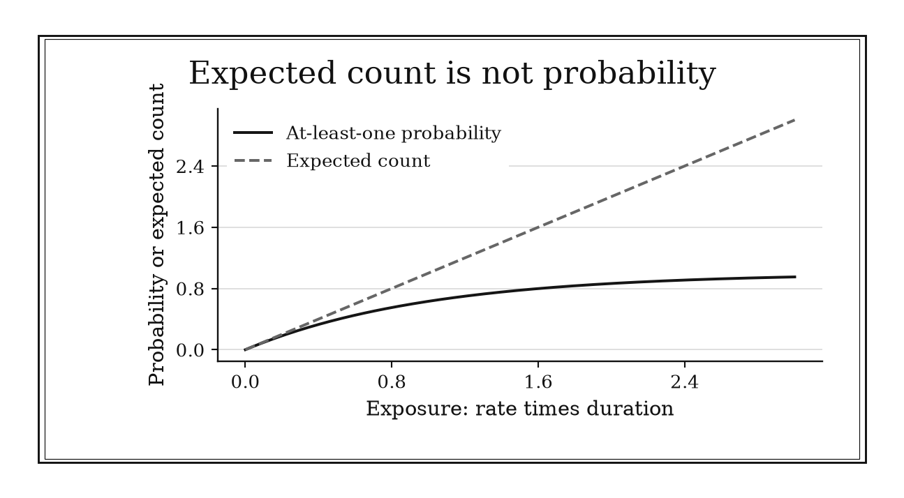
Figure 14.1. In a Poisson model, at-least-one probability is 1-exp(-exposure). At exposure one, it is about 0.632. Expected count equals exposure and can exceed one; probability cannot.
14.1.3: Mean Exponential Wait Is the Inverse Rate
History
A 1909 monograph titled The Theory of Probabilities and Telephone Conversations turned out to be an engineering tool disguised as a probability paper. Agner Krarup Erlang wrote it while working for the Copenhagen Telephone Company, modeling random call arrivals so engineers could size switching capacity for a fast-growing network. Treating call gaps as exponential waits, with the mean the inverse of the arrival rate, was the simplest payoff: a company could translate a measured rate directly into seconds worth planning around.
The equation
For an exponential waiting time with rate ,
and
Its median is .
How to read it
A rate and a mean wait describe the same memoryless arrival clock: a Poisson process, events occurring independently at a constant rate. Here is that rate and is the mean time to the next event; doubling events per hour halves the mean wait.
The mean is not the most likely wait, and it is not a deadline. Exponential waiting is right-skewed: most gaps are shorter than the mean, but occasional long silences pull the average past the median. The survival formula, , answers a different question: the chance a wait exceeds a chosen duration.
How to use it
A courier dispatcher fields pickup requests arriving at a steady six per hour, and a new driver wants to know how long to expect between pings before accepting a short side errand. Mean wait is hour, or 10 minutes, while the median is only about minutes; the probability of waiting more than 20 minutes is
About one ping in seven leaves a gap that long, so a 20-minute errand is a real gamble, not a safe bet just because the average gap is shorter.
Before trusting the estimate, the dispatcher should match units and check whether requests are genuinely steady rather than bunched around lunch and evening rushes; a rate that swings by time of day breaks the constant-rate assumption. This is an Independent rule: a credible constant arrival rate directly gives the mean and survival law for the next wait.
14.1.4: Memorylessness Means No Aging
History
A maintenance budget depends on one fact: whether an aging part carries more risk than a new one, and for a narrow class of processes, elapsed time carries no such information. At McGill University in 1902 and 1903, Ernest Rutherford and Frederick Soddy developed the transformation theory of radioactivity, establishing that each unstable species decays at its own exponential rate, with half-life a way to compare species and date materials. The memoryless label came later, not Rutherford or Soddy’s phrase; what they supplied was the decay data that made it unavoidable.
The equation
For an exponential lifetime ,
Equivalently, its survival function satisfies
The geometric distribution is the discrete-time counterpart.
How to read it
For a lifetime with this property, conditioning on survival past time leaves the remaining wait with the same distribution as a fresh one: . The clock does not remember how long it has run; expected remaining life stays at any age.
This property is unusual, not typical: among all continuous positive waiting times, the exponential is the only one with it. Most engineered parts have a hazard, the instantaneous chance of failure right now, that rises with wear or hides unobserved differences between units; nothing here tells you which is happening.
How to use it
A plant reliability engineer is deciding whether to swap out an industrial furnace igniter after it has run hours without failing, given a quoted mean life of hours under a constant-hazard model. Memorylessness says expected remaining life is still hours, the same as new; the completed 100 hours do not get subtracted to leave 400. Swapping it out early buys no reliability gain, only the cost of a new part.
The engineer should first check whether a constant-hazard model is defensible: an igniter degrading with heat cycling shows a rising hazard, and treating its age as irrelevant means running it past the point real wear has taken hold. Radioactive material fits the ideal closely; an aging igniter usually does not. This is an Independent rule: memorylessness alone lets elapsed waiting be discarded without changing the remaining-time calculation.
14.1.5: Superposed Poisson Rates Add
History
A dispatcher who assumes three merged call lines behave exactly like one line can badly misjudge how bursty the combined traffic is, especially if the streams are not actually independent. In 1940s Stockholm, Conny Palm developed point-process theory studying fluctuating telephone demand, and the Palm-Khintchine perspective explained why merging many sparse renewal streams can approach ordinary Poisson traffic, events scattered randomly at a steady rate. The exact case, where every component is already an independent Poisson process, sits inside that program as its cleanest case, exact rather than approximate.
The equation
For independent Poisson processes with rates ,
is Poisson with combined rate
How to read it
Expected events per unit time add like ordinary rates: if are independent Poisson processes with rates , their sum has rate . Independence and the Poisson structure survive the merge too: the combined stream keeps its Poisson character on every interval, a guarantee beyond matching means.
The exact theorem needs its streams to already be Poisson and independent. Palm’s broader result explains why a combined stream can approach that ideal even when no single source is Poisson alone, but that approximation carries its own conditions.
How to use it
A 911 dispatch center merges three independent regional call lines running at three, five, and two calls per minute, and a shift supervisor wants a single staffing estimate for the combined board. Adding rates gives calls per minute, and over a two-minute window the combined count is Poisson with mean and standard deviation . That merged number lets the supervisor plan staffing around one stream instead of three.
Before trusting the sum, the supervisor should confirm the lines can plausibly be treated as independent: a citywide power outage or a severe storm can drive spikes on all three lines at once, producing bursts far beyond what a Poisson model with rate 10 predicts. Merging also differs from splitting calls across specialty teams afterward; adding rates combines streams, it does not divide one. This is an Independent rule: independent Poisson streams can be replaced by one Poisson stream whose rate is their sum.
14.1.6: Poisson Thinning Multiplies the Rate
History
Independence survives even after a traffic stream is split by a fixed random rule: each destination still receives orderly traffic, related to the original only by a slower rate. Erlang’s Copenhagen telephone model, met earlier in this chapter, let engineers reason about capacity across trunks and exchanges from 1909 onward, and splitting a selected share of calls toward one line is natural in that setting. The modern thinning theorem formalizes the split; the record does not show Erlang proving it himself.
The equation
If each arrival in a rate- Poisson process is independently retained with probability , then
while
The two resulting processes are independent.
How to read it
If each arrival in a rate- Poisson process, independent events at a steady rate, is independently kept with probability , the kept stream is Poisson with rate and the dropped stream is Poisson with rate . Random labeling multiplies the rate by each label’s probability, the way sorting a deck by suit keeps every suit’s count random but shrinks its average.
Conditioned on the total count, the kept and dropped counts split like a coin flip per event. Averaged over the unknown total, the two streams turn out fully independent, stronger than sharing uncorrelated means, and easy to overlook.
How to use it
A retail loss-prevention analyst reviews a payment stream at transactions per hour and flags for manual review using an automated risk score. Thinning gives a flagged stream at per hour and an unflagged stream at per hour, both independent Poisson processes. That split lets the analyst staff the review queue around 20 cases per hour rather than the full 100.
The estimate depends on each transaction’s flag probability being stable and independent. A promotional sale can drive a surge of unusual purchases the risk score flags more often, raising the effective flagged rate above 20 even though the stated never changed. The analyst should track the flagged fraction hour by hour rather than assume it holds constant across a busy weekend. This is an Independent rule: independent random labeling converts one Poisson rate into category rates by multiplication.
14.1.7: Poisson Arrival Times Are Uniform Given the Count
History
It is tempting to credit Erlang with a calculation he never actually wrote down. That 1909 Copenhagen model, which also anchors the call-gap and thinning results elsewhere in this chapter, described traffic through Poisson counts, tallies of independent events at a steady rate, within fixed intervals. Once a homogeneous model is trusted and an interval’s total count is known, no single instant is privileged over any other, and sorting independent uniform draws to place those calls in time follows as an exact consequence of his setup, useful for simulating traffic he could only tabulate by hand.
The equation
Conditional on exactly arrivals by time ,
has the distribution of the sorted values of
How to read it
Conditioned on exactly arrivals by time , their unsorted locations behave like independent draws from a uniform distribution on , every instant equally likely. Sorting those draws gives the arrival times in order.
This does not say gaps between Poisson arrivals are uniform when the count is unknown; unconditionally, those gaps are exponential, as in the wait-time rule elsewhere in this chapter. The uniform statement holds only once interval and total count are fixed, and after sorting, the ordered times are no longer independent: an early arrival constrains room left for the ones that follow.
How to use it
A field ecologist knows a motion-sensor camera recorded exactly four animal sightings during a 60-minute window and wants to simulate plausible sighting times for a habitat model without rerunning the camera’s raw exponential-gap data. Drawing four independent values from and sorting them, say , , , and minutes, produces a conditional simulation consistent with the count.
The technique assumes a genuinely homogeneous sighting rate. If sightings cluster near dawn feeding times, the true process is nonhomogeneous, and uniform placement would spread sightings too evenly to match the real pattern. The ecologist would need to transform time through cumulative sighting intensity first, and if animals avoid or follow each other, even that falls short. This is an Independent rule: a fixed homogeneous Poisson count turns event-time simulation into sorting independent uniform draws.
14.2: Scaling and Memory Across Time
Randomness accumulates according to structure. Independent, centered increments spread on a square-root scale. Persistent processes recycle earlier shocks and can retain initial conditions far longer than a raw sample count suggests. These rules translate step size, diffusion, autoregressive coefficients, smoothing weights, renewal variability, and spectral gaps into interpretable time scales.
14.2.1: Random-Walk Displacement Grows as Root N
History
How far does a wanderer taking equal-length steps in random directions end up from home? In 1905, Karl Pearson posed that question to readers of Nature. Lord Rayleigh replied that essentially the same mathematics had appeared in his own work on random waves. Their exchange, a statistician’s puzzle meeting a physicist’s existing theory, made visible how a random walk’s spread scales: net displacement grows with the square root of the step count, not the full distance walked.
The equation
For independent steps with
the sum satisfies
How to read it
For independent steps with and , the sum , the total displacement of a random walk (a path built from independent random steps), has standard deviation . Positive and negative steps cancel on average, but their variances still add, so after steps the typical net distance grows only as fast as , even though the total path length grows as fast as itself.
Root- describes a typical scale of wandering, not a hard ceiling; a particular walker can end up much farther out. A nonzero average step size adds drift, a steady directional push layered on the random wandering, and drift eventually dominates root- fluctuation however small it is per step.
How to use it
A portfolio risk analyst tracks a strategy whose minute-by-minute tracking error behaves like a symmetric random walk with a typical step of percentage point, and a client wants cumulative deviation after 10,000 trading minutes. Standard deviation of net displacement is percentage-point-units, even though the sum of all moves along the path is 10,000 units; mistaking the second for the first would overstate expected drift.
Before trusting that estimate, the analyst must check whether the minute-by-minute steps are really centered at zero: a small, persistent bias adds a drift term that grows linearly and eventually swamps the fluctuation. Positive correlation between consecutive steps would also make the spread grow faster than predicts, so the analyst tests for both before reporting the flat root-time estimate as expected scatter. This is an Independent rule: independent mean-zero increments immediately determine a root- displacement scale.
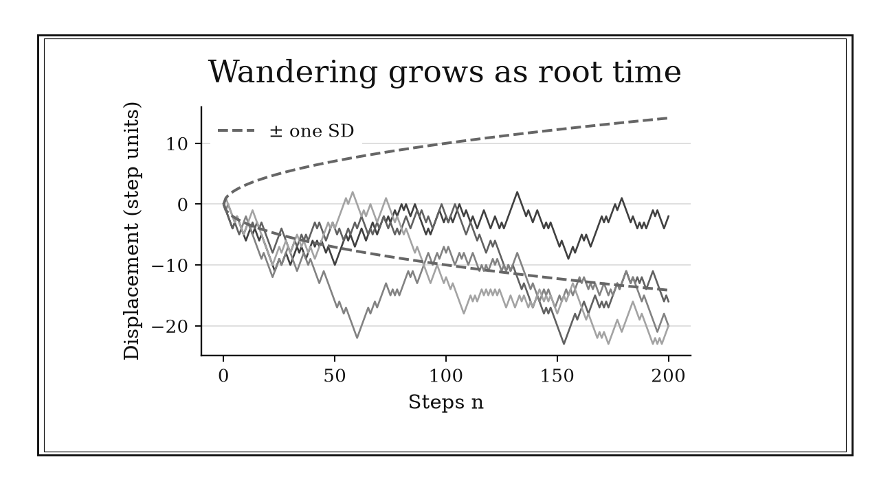
Figure 14.2. Four simulated symmetric walks illustrate paths around zero. The dashed ±sqrt(n) curves mark one standard deviation, not a boundary; individual paths cross them.
14.2.2: Diffusion Distance from (2Dt)
History
A 1905 theoretical paper made an oddly testable prediction about grains of pollen jittering under a microscope: their mean-square displacement should grow in direct proportion to time. Albert Einstein connected that jittering, Brownian motion, to molecular diffusion, and from 1905 to 1909, Jean Perrin tracked microscopic particles in Paris to test the claim, using the result to estimate Avogadro’s number. Perrin’s tracking turned an abstract prediction into an argument that helped settle whether atoms were real.
The equation
In one dimension,
so
In dimensions,
How to read it
In one dimension, mean squared displacement after time is , where is the diffusion coefficient, distance squared per unit time. Taking the square root restores distance, so RMS displacement is : it grows with the square root of time, not in direct proportion. In dimensions the analogous quantity is .
RMS distance is not the average signed displacement, which is zero for unbiased diffusion, and it is not a boundary containing every particle; it summarizes a spread with real probability on both sides. Because distance scales as , quadrupling elapsed time only doubles characteristic distance, so reaching twice as far takes about four times as long.
How to use it
A food scientist salting a batch of cured meat models salt diffusion with a coefficient and wants the characteristic penetration depth after seconds of brine contact before setting a cure time. One-dimensional RMS penetration is
roughly a centimeter, giving the scientist a characteristic diffusion scale for comparison with the cut’s thickness. A minimum cure time requires a concentration target, geometry, and boundary conditions; RMS displacement alone does not determine it.
To reach twice that depth, 20 millimeters, the scientist cannot simply double the time: since distance scales as , the required soak time roughly quadruples to about 400 seconds. The estimate also assumes diffusion alone is at work; if brine is actively pumped or massaged into the meat, that directed movement is advection, not diffusion, and it can carry salt in far faster than this formula predicts. This is an Independent rule: a diffusion coefficient and elapsed time directly produce the characteristic Brownian spread under the ordinary diffusion regime.
14.2.3: AR(1) Shock Half-Life
History
Mistake a temporary shock for a permanent shift in a persistent series, and a forecast can stay wrong for years after the disturbance has faded. In 1927 at Cambridge, G. Udny Yule modeled Wolfer’s annual sunspot numbers as a stochastic autoregression, treating each year’s count as depending on earlier years plus a fresh disturbance rather than a perfect cycle obscured by error. Yule’s model was second-order, not the single-coefficient AR(1) case here; the half-life formula, , translates an abstract coefficient into a duration anyone can picture.
The equation
Consider the AR(1) model
A shock remaining after periods is multiplied by . Its magnitude halves at
How to read it
In the model , a disturbance surviving periods is multiplied by each step, geometric decay. Solving for where that multiplier reaches one half gives the half-life, : a coefficient near zero forgets a shock almost immediately, one close to one retains it for many periods.
After two half-lives, one quarter of the shock remains; after three, one eighth. For negative , the sign alternates while its size still decays according to , so half-life describes the shrinking magnitude of a disturbance, not the direction the series is moving. The formula also says nothing about whether AR(1) itself is an adequate description of the series.
How to use it
A commodities analyst fits a monthly AR(1) model to a price series and finds , then needs to tell a trading desk how long a one-time supply shock will linger before deciding whether to hedge through it. Half-life is
months, so roughly three months after the shock, half its size remains, and after six months, about a quarter. Had the fitted coefficient instead been , the same shock would linger for about 13.5 months, a very different hedging horizon from the same-looking model.
The analyst must name the sampling interval: 0.8 means something different in daily, monthly, and annual data. Estimates of near one are unstable, since small fitting changes swing the half-life considerably, and a structural break in the market would make any single decay number misleading regardless of precision. This is an Independent rule: within a stable AR(1) model, one coefficient directly translates shock persistence into an interpretable half-life.
14.2.4: AR(1) Long-Run Variance Amplification
History
A persistent series’ current volatility is easy to mistake for only its latest shock, an error making any variance estimate run too small. Yule’s 1927 sunspot model, already the source of this chapter’s shock half-life, carried a second lesson: variability at any moment is the accumulated residue of many past shocks layered together, well beyond the newest one alone. Yule’s model was second-order, so the AR(1) variance formula here is a later simplification, while shock accumulation itself is the documented mechanism.
The equation
For
with innovations uncorrelated over time and with the process’s past, and with variance ,
How to read it
In with and innovation variance , the current value is a weighted sum of past innovations, and their variances form the series . Persistence amplifies shock variance into a larger level variance; since it uses , the sign of does not change its strength.
The amplification rises sharply as approaches one: at , the factor is , so a modest innovation supports a level ten times more variable than the shock itself. The formula cannot distinguish genuine persistence from apparent persistence caused by a shifting mean.
How to use it
A coach wants to know how much shooting variation is normal for a player before reacting to a hot stretch, so a basketball staffer fits an AR(1) model to efficiency deviations and estimates with innovation standard deviation percentage points. Stationary variance is
so the long-run standard deviation is about points, noticeably larger than the -point innovation standard deviation alone.
The coach should not mistake that -point swing for the player’s typical range: the figure already includes the accumulated effect of past variation. The estimate also requires and stable form across the season; a change in role or health partway through would break the constant-coefficient assumption this figure depends on. This is an Independent rule: stationary AR(1) persistence directly converts one-step shock variance into long-run level variance.
14.2.5: EWMA Effective Window Length
History
Give a control chart a fading memory instead of a short one, and it can catch a slow shift a chart reacting only to the latest reading would miss. In 1959, S. W. Roberts introduced the exponentially weighted moving-average chart in the United States, retaining every earlier measurement with geometrically decreasing weight rather than reacting mainly to the newest point, as a Shewhart chart does. The effective-window formula is a modern interpretation of that design.
The equation
For , after initialization effects have decayed, consider the long-running EWMA
Its normalized observation weights are . Their variance-equivalent sample size is
How to read it
For a smoothing weight between 0 and 1, each new observation gets weight and the running average carries forward weight . Matching that variance to a plain equally weighted average gives an effective window, , roughly when is small.
This is not a hard lookback with a sharp edge. Every past observation keeps some nonzero weight forever; “window” describes variance equivalence, not the age of the oldest value counted. A smaller gives a longer, quieter window; a larger reacts fast but stays noisier.
How to use it
A quality engineer running an EWMA chart on a filling line sets a smoothing weight and wants to explain how many recent fills the chart effectively “remembers” when judging whether a small shift is real. Effective window is
so the chart behaves like an average of the last 19 fills, smoothing noise while still reacting within a few dozen readings. Tightening to would stretch that memory to 99 fills, quieter but slower to flag a real shift.
The engineer should remember this window assumes independent, equal-variance noise between fills: autocorrelated fill weights or a genuine upward trend in target weight will distort what the chart’s memory represents, making the 19-fill figure a planning guide rather than an exact lookback. This is an Independent rule: under independent equal-variance noise, the smoothing weight directly yields a variance-equivalent number of observations.
14.2.6: Renewal Count Mean and Variance at Long Times
History
Not every stream of repeated waits arrives with no memory of what came before, and Conny Palm’s doctoral research pushed the mathematics past that special case. Working in Stockholm, Palm’s 1943 thesis on telephone-traffic intensity helped establish renewal theory: interarrival times sharing a common distribution without being forced exponential. A later theorem, not from Palm’s thesis, turns that generality into the long-time normal approximation used here.
The equation
For iid interarrival times with mean and variance , the renewal count at a long horizon satisfies approximately
Thus its approximate standard deviation is .
How to read it
For interarrival times drawn independently from a common distribution with mean and variance , the renewal count by a long time is approximately normal, . The mean count is horizon divided by average wait; the variance, more surprising, scales by but divides by , extra power needed to convert elapsed-time uncertainty into count uncertainty.
A renewal process, where each completed wait restarts the clock, need not have exponential waits or a mean equal to its variance, unlike Poisson. When waits are exponential, and the formula reduces to .
How to use it
At a repair shop where each job restarts the clock, a fleet manager schedules loaners around completions with mean repair time minutes and variance square minutes, over a -minute shift. Expected completions are , and the variance is
giving a standard deviation of . The manager plans coverage around completions rather than treating 100 as a fixed target.
This approximation only holds when the shift is long relative to a single repair and repairs are independent. A single stuck repair can distort the early part of the shift enough that the approximation misses the actual count; the manager should treat the estimate as a planning figure and verify it against a season of logs. This is an Independent rule: long-run wait moments directly forecast renewal count level and uncertainty.
14.2.7: Markov Mixing Scale from the Second Eigenvalue
History
Ranking billions of web pages by importance is a fixed point a computation converges toward, and reaching it is not automatic. At Stanford in 1998 and 1999, Larry Page, Sergey Brin, Rajeev Motwani, and Terry Winograd modeled an idealized web surfer as a Markov chain, a process jumping between states where each jump depends only on the current page, computing PageRank by repeated matrix multiplication. Teleportation handled dead ends and disconnected components. The original reports tracked convergence directly; reading it through the second-largest eigenvalue is a modern interpretation.
The equation
Let
For a finite reversible ergodic chain, the relaxation scale is
When , shrinking the slow mode to fraction requires roughly
How to read it
Let be the largest eigenvalue magnitude among the chain’s nonstationary modes, the vibration patterns that fade, rather than the one persisting at eigenvalue one, the stationary distribution, the long-run share of time in each state once settled. The relaxation scale is : a near one signals slow forgetting, a small one signals fast settling.
Shrinking the slowest mode to a fraction takes roughly steps, a useful forecast, not a guaranteed bound: constants depend on the starting state and the smallest stationary probability.
How to use it
A search-ranking engineer models a recommendation graph as a Markov chain and estimates its second-largest eigenvalue at , needing an iteration count before a ranking update is safe to publish. Reducing the slowest mode to one percent takes about
iterations, a starting horizon before checking convergence empirically. A competing graph with needs only about iterations for the same tolerance, so the first graph mixes slower.
Before trusting either estimate, the engineer must confirm the graph is reversible and every page can reach every other, since disconnected clusters never forget where they started. Huge graphs rarely expose their full spectrum, so the estimate is treated as a planning figure alongside trace diagnostics rather than a certified bound. This is an Independent rule: under the stated finite reversible-chain assumptions, the dominant nonstationary eigenvalue directly forecasts the slowest mixing scale.
14.3: Flow Systems and Simulation Guardrails
Flow systems can have finite average input but no stable long-run inventory. Simulations can store thousands of draws but contain only hundreds of independent-equivalent observations. This final family checks existence before using steady-state formulas, quantifies the price of operating near capacity, and treats MCMC output as a dependent time series rather than a spreadsheet of iid rows.
14.3.1: Little’s Law: Inventory Equals Throughput Times Time
History
A short 1961 paper in Operations Research settled an equation practitioners had already used for years without general justification. John D. C. Little supplied the missing proof that average inventory equals throughput times average time in system, , holding under broad steady-state conditions well beyond the narrow cases verified by hand. That proof turned a trusted rule of thumb into a theorem safe for any conserved flow system sharing its assumptions.
The equation
For a stable system with consistently defined boundaries,
For queue-only quantities,
Here is average inventory, is effective throughput, and is average time inside the same boundary.
How to read it
Over a long window, total customer-time inside a system can be measured two ways: as area under the curve of how many are present at each moment, or as the sum of every individual’s own time inside. Dividing both totals by the horizon gives average inventory, . The summed durations divided by the number of completions give average time , while completions divided by the horizon give throughput ; together these yield once boundary effects vanish.
The law needs no particular arrival pattern or service-time distribution; its power comes from conservation, not a specific model. Two systems can share the same , , and while one makes every customer wait nearly the same time and the other has most wait briefly and a few wait very long.
How to use it
A hospital patient-flow coordinator tracks an emergency department that discharges or admits 12 patients per hour, each spending half an hour from arrival to disposition, and needs a working estimate of occupancy for a staffing request. Little’s law gives
patients in the department on average, a figure to hand administration as expected occupancy under current flow.
Before using that number to plan bed counts, the coordinator must be careful which time is measured: if only time waiting for a bed counts, the queue-only version applies instead, and mixing the two would misstate occupancy. The law also assumes today’s flow is representative; a surge in walk-ins or boarded patients awaiting beds would push occupancy past what this average predicts, since the identity is silent on how long any individual patient waits. This is an Independent rule: conservation directly relates average inventory, throughput, and time across queues, factories, hospitals, and other stable flow systems.
14.3.2: M/M/1 Stability Requires Utilization Below One
History
Stability on paper is not comfortable service, and that gap is the stake behind checking utilization before trusting any steady-state formula. From 1909 through 1920, Erlang’s Copenhagen teletraffic work, behind this chapter’s call-gap and thinning rules, turned statistical equilibrium into an engineering capacity requirement: enough lines and operators had to exist for the rate observed. His exchanges ran many circuits at once; is the modern statement for the single-server version.
The equation
For Poisson arrivals at rate and exponential service at rate ,
An M/M/1 queue has a finite stationary distribution only when
How to read it
Utilization compares incoming work, arrivals per unit time , against capacity, completions per unit time . An M/M/1 queue, a single server with Poisson arrivals (independent events at a steady rate) and exponential service, settles into a stable pattern, its stationary distribution, only when ; otherwise backlog has nowhere to settle.
Passing that check is not comfortable service. A just under one leaves almost no spare capacity to absorb a busy stretch. In the standard model, equals the fraction of time the server is busy, so is the capacity margin, worth watching as closely as stability.
How to use it
A city 311 call center manager fields nine calls per hour while a single operator can close out ten per hour, and the manager wants to know whether current staffing is sustainable before a budget review cuts one shift. Utilization is
so the textbook model is stable, technically, but with very little slack: the operator is busy 90 percent of the time, leaving only a 10 percent margin to absorb any unusual morning.
If call volume rises to ten per hour, matching the operator’s rate, the steady-state formulas this rule gates stop applying: queue length grows without ever settling, very different from a large but finite queue. Treating as only a slightly worse version of badly understates what has changed. The manager should read near one as a signal to add capacity, not as confirmation that staffing works. This is a Workflow heuristic: it gates all steady-state M/M/1 calculations by checking whether a stationary regime can exist.
14.3.3: M/M/1 Delay Blows Up Near Capacity
History
A planner who sizes a phone system for average call volume alone can still watch hold times spiral once traffic nudges just above average. Erlang’s Copenhagen queueing analysis returns to this chapter one rule later with its sharpest warning: average load hides congestion near full capacity. He studied mostly multiserver systems; the single-server formula here, , is a later expression of that lesson, not his own analysis.
The equation
For a stable M/M/1 queue,
and mean waiting time before service is
How to read it
Mean time in system is , and mean wait before service alone is . The spare-capacity margin, , sits in the denominator, so each increment of utilization costs more delay, and mean time grows without bound as approaches one.
Stability is only the first question; how far a system sits from that boundary determines whether delay is mild or severe. The difference between and is the mean service time, . Averaging over a long period can hide a daily peak behaving like a much more loaded queue.
How to use it
A customer-support call center handles 8 calls per hour against a service rate of 10 per hour per agent line, and management wants to know what happens to hold times if a marketing push raises call volume to 9 per hour. At the current load, mean time in system is
30 minutes; raising arrivals to 9 per hour gives
doubling mean time in the system from a rate increase of just
12.5 percent, because the spare margin has fallen from two calls per hour to one.
Management should present that comparison to justify adding a second agent line before the push begins rather than after hold times spike. The formula assumes exponential service and a single line; nonexponential service times would change the exact numbers, though the lesson that delay worsens sharply near capacity tends to survive. This is an Independent rule: in a credible M/M/1 model, the capacity margin directly prices mean delay and exposes near-capacity blow-up.
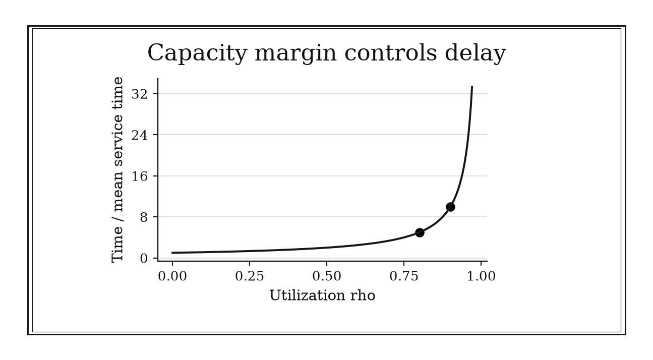
Figure 14.3. For an M/M/1 queue, mean time in system measured in mean-service-time units is 1/(1-rho). It doubles from five to ten as utilization rises from 0.8 to 0.9.
14.3.4: MCMC Effective Sample Size from Autocorrelation
History
Ten thousand stored samples from a correlated simulation can carry the statistical weight of only a few hundred independent observations, a consequence of how Markov chain Monte Carlo methods generate draws. In 1953 at Los Alamos, Nicholas Metropolis, the Rosenbluths, and the Tellers used the MANIAC computer to simulate interacting particles, updating one configuration from the previous one rather than drawing each new state fresh. That made high-dimensional simulation practical, but produced a correlated sequence. Effective sample size is a later diagnostic for that dependence, not reported in the original paper.
The equation
For a stationary chain satisfying a central-limit theorem and an estimand whose lag autocorrelations have a convergent sum,
and approximately
How to read it
Nearby draws in a correlated chain, where each new value depends on the one before, are partly redundant rather than fully independent. Summing the chain’s autocorrelations, its lag-by-lag tendency for one value to track the last, gives an integrated autocorrelation time , and dividing the draw count by gives the effective sample size, .
Effective sample size belongs to one estimand at a time: a sampler can estimate a central average efficiently while exploring a tail probability poorly, so one reported gives no information about the precision of another quantity.
How to use it
A graduate researcher runs a Bayesian model, retains post-warm-up draws, estimates the integrated autocorrelation time at , and needs a defensible standard error for a thesis committee. Effective sample size is
so the Monte Carlo standard error is times larger than the naive formula using all ten thousand rows would suggest, and the researcher reports precision based on 500, not 10,000, draws.
Working backward, if the committee wants an effective sample size of and holds, the chain needs roughly retained iterations, a useful planning number. The researcher should also check autocorrelation for any tail quantile, since a healthy central does not confirm the sampler explored every mode. This is a Workflow heuristic: it replaces nominal MCMC length with estimand-specific independent-equivalent information before precision is reported.
14.3.5: Burn In for Several Dependence Time Scales
History
No fixed percentage of a run can honestly answer how many discarded iterations are enough to call a chain warmed up, and the 1953 Los Alamos Metropolis simulation, the same MANIAC experiment behind this chapter’s effective-sample-size rule, shows why: the chain began from a constructed arrangement and had to move toward thermal equilibrium before its measurements represented the target. The paper never named it “several dependence time scales”; it left the harder task: discard enough iterations that the chain forgets where it started.
The equation
If a slow discrepancy decays approximately as , then reducing it to fraction requires
For , both logarithms are negative and the result is positive.
How to read it
If a slow diagnostic quantity decays roughly like , reducing it to a fraction of its initial size takes about iterations. Warm-up needs to cover enough of that decay, in the chain’s slowest mode, that the starting point’s influence becomes negligible relative to the precision needed.
A fixed percentage of run length carries no general meaning: two chains can forget their starts on entirely different time scales. This formula is a planning approximation for one geometric decay, not a certificate of convergence; some unmonitored aspect of the target may relax far more slowly than whatever summary is being watched.
How to use it
A statistician planning an MCMC run estimates the chain’s dominant persistence at and needs a defensible warm-up length before a report is due. Reducing an initial discrepancy to one percent takes about
iterations, so the statistician budgets at least that many discarded draws, and checks that after only ten iterations roughly
35 percent of the initial discrepancy would still remain, far too much to trust.
Before finalizing that budget, the statistician starts several chains from overdispersed points and confirms convergence to the same summaries, since no fixed discard length proves convergence on its own. A multimodal posterior can defeat the geometric picture; discarding more iterations will not fix a chain stuck in the wrong region, and between-chain diagnostics are the actual check. This is a Workflow heuristic: estimated relaxation controls a first warm-up budget, while multiple-chain evidence decides whether initialization has actually been forgotten.
14.3.6: The 0.234 Random-Walk Metropolis Benchmark
History
Tuning a random-walk proposal by feel leaves a sampler crawling or flailing, and in 1997, Gareth Roberts, Andrew Gelman, and Walter Gilks gave that guesswork a number. Working in the United Kingdom and the United States, they proved a weak-convergence result for random-walk Metropolis on high-dimensional, smooth, product-shaped targets. Optimizing the resulting diffusion’s speed produced an asymptotic acceptance rate near , with its narrow assumptions part of the result, not fine print set aside once the number is remembered.
The equation
Under the diffusion-limit assumptions, proposal scale is
and as dimension grows,
How to read it
A random-walk proposal, a candidate step drawn by adding random noise to the current position, too large travels farther when accepted but gets rejected more often; one too small is accepted almost every time but barely moves the chain. The theorem behind balances squared travel distance against acceptance probability in a smooth, high-dimensional regime.
The number describes a benchmark for one algorithmic geometry, not a definition of a well-tuned sampler: acceptance rate alone does not measure mode exploration. Proposal size should also shrink roughly as as grows, and describes the balance reached only after that shrinking has happened.
How to use it
During a diagnostic run for a smooth, high-dimensional posterior, a Bayesian modeler tuning a random-walk Metropolis sampler observes an acceptance rate of and must decide how to adjust the proposal. That low rate signals proposals are usually far too large, since the theorem’s setting predicts a healthy rate near ; the modeler shrinks the scale and re-checks, aiming for the broad range to rather than chasing exactly.
The modeler should not carry that target into a different sampler: for Gibbs sampling, Hamiltonian Monte Carlo, discrete states, or a one-dimensional target, the theorem’s assumptions do not hold, and reparameterizing the model matters more than matching one number. Effective sample size per unit of computing time should judge sampler quality, with used only as a narrow starting diagnostic. This is a Workflow heuristic: it supplies a scoped tuning diagnostic for high-dimensional random-walk Metropolis, with its asymptotic assumptions kept attached.
Chapter Synthesis: Match the Time Scale to the Question
Stochastic-process shortcuts become reliable when their clocks and assumptions are named. A homogeneous Poisson rate creates a coherent family: rate times exposure gives a count scale, the zero-count complement gives event risk, inverse rate gives mean waiting, and superposition or thinning modifies rates predictably. Conditional on a fixed count, uniform order statistics place the events. Memorylessness belongs to this constant-hazard world and should not be exported casually to aging systems.
Across longer horizons, independent increments and persistent dependence behave differently. Random walks and diffusion spread on square-root scales because variances add. AR coefficients, EWMA weights, renewal moments, and Markov eigenvalues turn less visible dependence into half-lives, effective windows, count uncertainty, and mixing horizons.
Flow and simulation calculations require one further discipline: verify that a steady regime exists before using its averages. Little’s law links conserved throughput and occupancy broadly, while M/M/1 formulas require a much narrower model and become singular near capacity. MCMC output must be judged by warm-up, autocorrelation, and algorithm-specific diagnostics rather than row count.
Across all twenty rules, ask four questions:
- What is the exposure or observation interval, and are all rates expressed on it?
- Which independence, stationarity, and distribution assumptions create the shortcut?
- What time scale controls spread, persistence, mixing, or equilibration?
- Does a stable long-run regime exist, and is the reported precision effective rather than nominal?
One-Page Stochastic Processes Toolkit
| Recognition cue | Rule to try | What it gives | Role |
|---|---|---|---|
| Homogeneous rare-event rate and exposure | Count mean, variance, and scale | Independent | |
| Risk of any Poisson event | At-least-one probability | Independent | |
| Homogeneous arrival rate | Mean exponential wait | Independent | |
| Constant-hazard survival | Apply memorylessness | Remaining wait unchanged by elapsed time | Independent |
| Independent Poisson streams merge | Add | Combined Poisson rate | Independent |
| Events receive independent random labels | Multiply rate by | Thinned category rate | Independent |
| Poisson count fixed within an interval | Sort iid uniform times | Conditional arrival locations | Independent |
| Independent centered steps accumulate | Use | Typical net displacement | Independent |
| Brownian diffusion over time | Use | RMS displacement | Independent |
| AR(1) persistence must be communicated | Use | Shock half-life | Independent |
| AR(1) innovation and level variance differ | Divide by | Stationary variance | Independent |
| EWMA smoothing weight is abstract | Use | Variance-equivalent window | Independent |
| Nonexponential iid renewal waits | Use long-time renewal normal law | Count mean and variance | Independent |
| Finite reversible Markov chain mixes slowly | Inspect | Relaxation and mode-decay scale | Independent |
| Stable conserved flow system | Use | Inventory, throughput, or time | Independent |
| M/M/1 steady-state formula is proposed | Check first | Stability gate | Workflow |
| Single-server queue approaches capacity | Use | Mean delay blow-up | Independent |
| MCMC draws are autocorrelated | Use | Effective sample size | Workflow |
| MCMC start may still matter | Budget several relaxation scales | Warm-up plan and diagnostic | Workflow |
| Random-walk Metropolis is being tuned | Apply only in scope | Proposal-scale benchmark | Workflow |
Decision Path
- Do you have a stable event rate and an exposure? Use for a Poisson count scale. Use the zero-count complement for event risk and for an exponential mean wait.
- Are event streams being combined or split? Add rates only for independent Poisson streams. Multiply by label probabilities only for eventwise-independent thinning.
- Is the total count fixed? Simulate homogeneous event locations as sorted uniforms; otherwise retain the exponential-gap view.
- Is randomness accumulating through independent centered increments? Expect root-time or root-step spread. Add drift separately and inspect dependence.
- Is a time series persistent? Translate into half-life and stationary variance only after checking and the adequacy of an AR(1) model.
- Is a smoother or renewal process being summarized? Convert EWMA weight to a variance-equivalent window, or wait moments to a long-horizon count approximation, while keeping their regimes explicit.
- Is a Markov chain being run? Estimate its slowest dependence scale, then use multiple-chain evidence and estimand-specific ESS rather than nominal iterations.
- Is a queue or flow system involved? Apply Little’s law with consistent boundaries. For M/M/1 calculations, establish before evaluating delay and preserve capacity headroom.
- Is proposed as a tuning target? Confirm high-dimensional random-walk Metropolis assumptions; otherwise use diagnostics appropriate to the actual sampler.
Transfer Problems
1. Separate Poisson count, risk, and waiting questions
A help desk receives homogeneous independent requests at three per hour. Over a two-hour interval, find the expected count, count standard deviation, probability of at least one request, and mean wait to the next request. Then state what extra conditioning allows six arrival times in that interval to be simulated by sorting uniform draws. Identify two observations that would challenge the homogeneous Poisson model.
2. Translate dependence into several time scales
A monthly AR(1) fit has and innovation standard deviation . Compute the shock half-life and stationary level variance. Compare the half-life with the roughly periods needed for a discrepancy to fall to one percent. Explain why these calculations do not establish that the fitted series or an MCMC chain has reached stationarity.
3. Diagnose a loaded queue and its simulation
An M/M/1 service system has and per hour. Compute utilization, mean time in system, and average inventory from Little’s law. A simulation stores post-warm-up draws with integrated autocorrelation time for mean delay. Compute ESS, then list the stability, warm-up, and between-chain checks needed before treating the result as trustworthy.
Where These Ideas Reappear
- Probability: Poisson counts, exponential waits, conditioning, renewal limits, and Markov chains connect static distributions with processes evolving in time.
- Statistics: overdispersion, autocorrelation, effective sample size, stationarity, and time-series persistence determine which uncertainty formulas remain valid.
- Differential equations and physics: diffusion equations, Brownian motion, relaxation modes, and radioactive decay translate microscopic randomness into macroscopic laws.
- Operations research: Little’s law, capacity margins, and congestion curves guide staffing, manufacturing, hospital flow, and network design.
- Computer science: PageRank, randomized algorithms, cache and request traffic, and Markov-chain simulation depend on mixing and rate models.
- Reliability and survival analysis: hazards, event risk, memorylessness, and nonhomogeneous intensities distinguish aging from constant-rate failure.
- Signal processing and quality control: EWMA memory, autoregressive variance, and shock half-life tune filters and monitoring systems.
- Bayesian computation: burn-in, ESS, and proposal tuning turn dependent MCMC trajectories into defensible estimates.
Historical Notes and Sources
The historical profiles distinguish original discoveries and applications from modern operational deductions. Several events deliberately support more than one rule: Bortkiewicz’s exposure table supports both Poisson count and zero-count calculations; Erlang’s traffic work supports rate, wait, thinning, conditional-time, and queueing interpretations; Yule supports two AR(1) specializations; and the Metropolis experiment supports later warm-up and ESS diagnostics.
- Bortkiewicz and Prussian horse-kick counts: Bortkiewicz’s 1898 book; Royal Statistical Society reanalysis.
- Erlang’s 1909 Poisson telephone model: bibliographic record for Erlang’s paper; INFORMS history of Erlang and queueing.
- Rutherford, Soddy, and exponential radioactive decay: APS historical account; Rutherford’s Nobel lecture.
- Palm, superposition, and renewal traffic: INFORMS discussion of Palm’s teletraffic role; INFORMS queueing history.
- Pearson, Rayleigh, and the random walk: Pearson’s 1905 Nature question; MIT notes on the Pearson–Rayleigh origin.
- Einstein and Perrin on Brownian displacement: APS history of Einstein’s Brownian-motion paper; Perrin’s Nobel lecture.
- Yule’s autoregressive sunspot model: Yule’s 1927 paper; Royal Society referee record; historical review of sunspot autoregression.
- Roberts and EWMA control charts: Roberts’s 1959 paper; NIST Engineering Statistics Handbook.
- PageRank and Markov iteration: original Stanford technical report; Stanford copy of the early Google paper.
- Little’s law: Little’s 1961 proof; Little’s Law at 50.
- Metropolis simulation, equilibration, and dependence: Metropolis et al. 1953; historical review of MCMC; Stan Reference Manual on effective sample size.
- The 0.234 random-walk Metropolis result: Roberts, Gelman, and Gilks, 1997; later discussion and generalization.