Chapter 15: Information Theory: Measuring Information and Its Limits
A sharpened photograph may look more informative than the original sensor image. A compressed representation may make a pattern easier for a classifier to use. Yet if no side information enters, neither operation can create new evidence about the scene that produced the original pixels. Processing can reorganize information, expose it, or destroy it. It cannot manufacture it.
Information theory turns statements like that into arithmetic. Probability becomes surprisal. Average surprisal becomes entropy or cross-entropy. Statistical dependence becomes mutual information. Communication and compression acquire limits that no clever implementation can exceed under the stated model.
The twelve rules in this chapter form three families. The first builds a numerical language for rarity, uncertainty, and predictive difficulty. The second measures dependence and the loss imposed by processing or distributional approximation. The third translates entropy into operational limits for noisy channels, prefix codes, and probabilistic membership structures.
The governing habit is: state the probability model and log base, then distinguish the information a representation contains from how conveniently a particular method can use it.
15.1: A Numerical Language for Information
The logarithm is the bridge from multiplicative probability to additive information. It turns one event’s rarity into bits, averages those bits into entropy, and converts predictive log loss into perplexity. Each quantity has a precise model and comparison domain.
15.1.1: Surprisal Is Minus Log Probability
History
A telegraph key at Bell Telephone Laboratories could select among several equally probable symbols, and each added selection multiplied the possible message sequences that might follow. In 1928, Ralph Hartley wanted a measure of information that ignored meaning and tracked only how many sequences remained possible. The multiplying possibilities called for a logarithm, turning products into sums so two independent selections would add their information instead of multiplying it. Claude Shannon later extended Hartley’s equal-probability count to unequal likelihoods. “Surprisal” is a later name for the quantity; the additive design was already Hartley’s.
The equation
For an outcome (x) with modeled probability (p_x>0), its base-2 surprisal is
For independent outcomes (x) and (y),
How to read it
Here (p_x) is the modeled probability of an outcome, and (I(x)=-_2p_x) converts it into bits, the units a base-2 logarithm produces. A common outcome, near probability 1, carries almost no surprisal; a rare one carries much more. Halving a probability adds exactly one bit, since (-_2(p/2)=-_2p+1). For independent outcomes, surprisal adds where probability would have multiplied: (I(x,y)=I(x)+I(y)). The number reflects only the stated model, not the outcome’s importance once it occurs.
How to use it
A warehouse manager comparing information scores for pallet conditions starts with a cold-chain breach flag of modeled probability (p=2^{-10}=1/1024). That outcome has surprisal (I=10) bits. Two independent outcomes with probabilities (1/8) and (1/32) have joint surprisal (3+5=8) bits. These are information scores and ideal coding costs, not mandatory lengths of individual codewords; actual prefix-code design uses the whole symbol distribution, as discussed later in this chapter. Frequencies drifting from the model change the scores, and an event assigned (p=0) has infinite surprisal, exposing an overconfident model rather than infinite importance. This is an Independent rule: a stated event probability directly determines its information score across coding, inference, and risk analysis.
15.1.2: Entropy Cannot Exceed Log Alphabet Size
History
Every channel has an absolute ceiling on how much a single selection can convey, and in 1928 Ralph Hartley set out to fix that ceiling for a telegraph choosing among (s) equally available symbols. Possible sequences for (n) selections numbered (s^n), a ceiling no coding scheme could exceed without changing the alphabet. Shannon’s 1948 entropy generalized Hartley’s count to unequal symbol probabilities: Hartley’s equal-choice case was the single distribution carrying the most uncertainty a fixed alphabet could hold.
The equation
For a discrete variable (X) on an alphabet of (M) possible symbols,
with (0=0). Equality holds when
How to read it
Entropy, (H(X)), is the average surprisal of a variable (X) across its distribution, in bits. On an alphabet of (M) symbols, entropy never exceeds (_2M), reaching that ceiling only when every symbol is equally likely. A biased alphabet always has less entropy than the uniform case, since predictability lowers average surprise. Doubling an alphabet from 4 to 8 symbols raises the ceiling from 2 bits to 3, not 4: it grows with the logarithm of size, not the size itself.
How to use it
A systems designer setting the alphabet for a four-character PIN wants an honest ceiling on its guessing resistance. Ten digits give at most (H_2 10) bits per character, so four independent, uniform digits cap out at (4) bits, matching (10^4=10{,}000) equally likely combinations. A 36-character set raises the ceiling to (_2 36) bits, about (20.7) across four, only if characters are uniform. If users pick digits themselves, choices like birthdays cluster far from uniform, so true entropy sits well under the ceiling despite the alphabet’s nominal size. The designer treats the ceiling as a best case. This is an Independent rule: alphabet size directly supplies a portable upper bound on discrete uncertainty and representational demand.
15.1.3: Entropy of a Rare Bernoulli Event
History
Drop the common symbol’s contribution from a rare-event entropy estimate and the result looks plausible while still being wrong. Shannon’s 1948 paper plotted the entropy of a two-symbol source against its symbol probability (p); the curve peaks for a fair source and collapses toward zero as one symbol becomes almost certain. That collapse has two sources: the rare term (-p_2p) and the common symbol, which still contributes a first-order share near (p). The small-probability estimate below reads that curve’s tail and keeps the term the shortcut drops.
The equation
For a Bernoulli event with probability (p),
As (p),
Equivalently, the leading pieces are (p_2(1/p)+p/).
How to read it
For a rare binary event with probability (p), entropy (H_2(p)), the average bits of surprise per trial, is close to (p_2(e/p)). The rare outcome contributes (p_2(1/p)), but the common outcome adds its own share, (p/), since its small surprisal is not zero. Both shrink toward zero as (p). This small-(p) approximation is unreliable near one half; use the exact entropy there. For (p) near one, apply the rare-event approximation to (1-p), since (H_2(p)=H_2(1-p)).
How to use it
A wildfire-sensor network reports a rare “ember detected” flag with modeled probability (p=0.01) per cycle, and an engineer wants the entropy budget for logging it. The approximation gives (p_2(e/p)=0.01_2(271.8)) bits, close to the exact (0.0808) bits: safe here. The naive (-p_2p) bits understates the average by roughly 18 percent, enough to under-provision a channel sized on it. The engineer budgets the fuller estimate and checks that cycles are close to independent: if embers cluster once a fire starts, the entropy rate across a session can run well below this figure. This is an Independent rule: after verifying a genuinely rare Bernoulli regime, it directly estimates average information per trial.
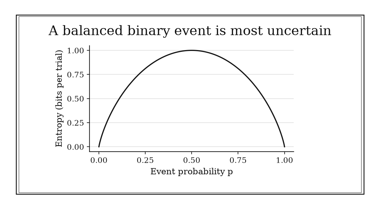
Figure 15.1. Binary entropy is symmetric, reaches one bit at p=0.5, and tends to zero at either endpoint. Use the exact curve outside the rare-event regime.
15.1.4: Perplexity Is Exponentiated Cross-Entropy
History
A one-bit improvement in a speech recognizer’s average prediction meant something concrete: half as many effectively likely next words at every step. That was the payoff Frederick Jelinek, Robert Mercer, Lalit Bahl, and James Baker were chasing in 1977 at IBM’s Thomas J. Watson Research Center, needing a fair way to compare speech-recognition task difficulty. Counting vocabulary size alone did not work, since possible next words were rarely equally likely. They introduced perplexity to convert that uneven uncertainty into a single branching factor, later restated as exponentiated average log loss in today’s cross-entropy notation.
The equation
For a sequence (x_1,,x_n) scored by predictive model (q), the base-2 empirical cross-entropy is
Perplexity is
With natural-log cross-entropy, the equivalent definition is (PP=e^{H_{}}).
How to read it
Cross-entropy (H_{}) is the average bits a model’s predictions cost per token, and perplexity reverses that scale by exponentiating: (PP=2^{H_{}}). A cross-entropy of (h) bits per token behaves, on average, like choosing uniformly among (2^h) options at every step, though real tokens rarely have that many live candidates; it is a geometric-mean statement, not a literal count. Each one-bit reduction halves perplexity outright. The number only means what it claims against the same tokenization and evaluation data that produced it.
How to use it
A speech-technology team compares two dictation models on the same evaluation set and needs a number a manager can grasp without decoding bits. Model A scores cross-entropy (5) bits per token, giving perplexity (PP=2^5=32). Model B reaches (4) bits, so (PP=2^4=16), half of Model A’s. The team recommends Model B. Before signing off, they confirm the two models share tokenization: switching to smaller subword units would lower perplexity on its own while whole-word prediction stays no better, and lower perplexity is not a promise about factual accuracy or calibration. This is an Independent rule: within a fixed evaluation setup, it directly translates additive predictive log loss into an intuitive multiplicative scale.
15.2: Dependence and Irrecoverable Loss
Correlation sees only a narrow kind of relationship. Mutual information tests the entire joint distribution against independence. Once information passes through a Markov chain, the data-processing inequality sets a one-way limit, while Pinsker turns one information discrepancy into a bound on every event probability.
15.2.1: Mutual Information as a Dependence Screen
History
Correlation can say two variables have nothing to do with each other while a deeper measure insists they are completely entangled, and Shannon’s 1948 communication theory supplied the tool that settles the disagreement. Shannon wanted to quantify how much observing a channel’s output reduced uncertainty about the sent message, turning “what did the receiver learn?” into a number. His mutual information compares the real joint behavior of two variables against the behavior they would show if independent. The modern KL-divergence form used below restates that question in a way that also catches dependence correlation cannot see.
The equation
For finite discrete variables,
Moreover,
How to read it
Mutual information (I(X;Y)) measures how far a pair of variables sits from acting independently: zero exactly when knowing (X) tells you nothing new about (Y), positive whenever it does, in bits. It equals the KL divergence between the joint distribution of (X) and (Y) and the distribution they would have if independent, so any departure from that product raises it above zero. Unlike correlation, which catches only straight-line relationships, mutual information catches curved and non-monotone dependence too, though it cannot identify which variable causes the other.
How to use it
A geneticist screens two markers, (X) and (Y), and a standard correlation test comes back at zero. Suppose (X) is uniform on ({-1,0,1}), three equally likely genotype codes, and (Y=X^2) tracks a trait present only when (X). Then (E[X]=0), (E[XY]=E[X^3]=0), so ((X,Y)=0): correlation reports nothing. But (Y) is determined by (X), with (P(Y=0)=1/3), (P(Y=1)=2/3), so (I(X;Y)=H(Y)=H_2(1/3)) bits, far from zero. The geneticist follows up the pair rather than discarding it on correlation. Finite-sample estimates are sensitive to binning, and a small measured value does not establish independence or rule out a relationship the estimator missed. This is an Independent rule: a valid joint distribution directly supplies a general dependence measure across channels, features, and data analysis.
15.2.2: Processing Cannot Create Information About the Source
History
Once a signal has passed through several stages, how much can anyone still say about the original source? Shannon’s 1948 communication diagram split that question into distinct pieces: a source, an encoder, a noisy channel, a decoder, and a destination, each stage acting only on what the previous stage handed it. The split let engineers ask what every transformation preserved or destroyed about the message. The data-processing inequality is the standard theorem following from this framework: without independent new evidence, no decoder can reveal more about the source than its input already carried.
The equation
If (XYZ) is a Markov chain, meaning
then
For a deterministic transformation (Z=g(Y)), the Markov condition holds automatically.
How to read it
If (X), (Y), (Z) form a chain where (Z) is built only from (Y), never touching (X), then (Z) cannot carry more mutual information about (X), dependence measured in bits, than (Y) already did: (I(X;Z)I(X;Y)). Once (Y) is known, (Z) gets no further evidence from (X). Processing can make existing information easier to use; it cannot manufacture new evidence about the source itself.
How to use it
An imaging team sharpens satellite photographs before handing them to an analyst and wants to know what that step can and cannot buy. Suppose the raw sensor image (Y) carries (3) bits of mutual information about the true ground state (X). Any downstream transform (Z=g(Y)), sharpening included, satisfies (I(X;Z)) bits: no processing step recovers detail the sensor never captured. Sharpening still helps by making those 3 bits easier to see, a real gain even though the ceiling has not moved. The team avoids claiming the sharpened image “contains more information,” since that phrase misstates what happened. If a second sensor is fused in later, the chain changes and new evidence can enter. This is an Independent rule: a verified source–representation–processing chain directly bounds what every downstream transformation can retain about the source.
15.2.3: Pinsker Converts KL Divergence to Probability Error
History
A 1953 doctoral thesis already contained the inequality the field would later name after someone else. Modern historical work shows Marco Schützenberger proved, in that thesis, the bound now associated with Mark Pinsker, including its optimal constant. Pinsker’s own 1960 work helped establish related bounds in information theory, but the familiar eponym conceals the earlier result. The inequality converts an abstract relative-entropy discrepancy, a divergence between two probability distributions, into a concrete bound on how far apart those distributions can be on any single event. Getting the origin right matters for the same reason the rule does: both trust a bound over a convenient story.
The equation
Define total variation by
in the discrete case. With natural-log KL divergence,
If KL is measured in bits, multiply it by () inside the square root.
How to read it
Total variation (|P-Q|{}) is the largest possible gap between two distributions’ answers to the same yes-or-no question about any event. KL divergence (D{}(P|Q)) measures how distinguishable (Q) is from a reference distribution (P), in nats under natural logarithms. Pinsker’s inequality says a small KL divergence forces total variation to be small too: (|P-Q|_{}). The implication runs one way: total variation can stay small while KL divergence is large, or infinite, if (Q) assigns near-zero probability somewhere (P) does not.
How to use it
A credit-risk analyst has fit a model distribution (Q) for default outcomes. Suppose an independently justified population guarantee gives (D_{}(P|Q)) nats for the true distribution (P). Pinsker then gives (|P-Q|_{}=0.10), so every event (A) has (|P(A)-Q(A)|). A KL estimate from backtesting alone would not certify that guarantee; its estimation uncertainty and unobserved tails must also be addressed. The implication runs only one way: a small total-variation gap would not bound KL, since (Q) could assign near-zero probability to a rare scenario (P) takes seriously. This is an Independent rule: a KL guarantee directly becomes a uniform event-probability guarantee in model approximation, learning, and inference.
15.3: Operational Limits and Design Rules
Information measures become most useful when they constrain an engineering action. A second-moment constraint creates a maximum-entropy distribution. Noise and power create channel capacities. Entropy brackets prefix-code length. A controlled false-positive trade permits a memory-efficient Bloom filter.
15.3.1: Gaussian Has Maximum Entropy at Fixed Variance
History
A communication-capacity calculation is only as good as its noise model, so Shannon needed to know which noise shape was truly the hardest case before trusting any capacity number. In his 1948 analysis, he used the fact that among continuous distributions sharing one fixed variance, the Gaussian carries the greatest differential entropy, the broadest possible spread of uncertainty. That made Gaussian noise part of a sharp, provable communication limit rather than a convenient stand-in. Fixing the average squared spread leaves shape otherwise free, and the Gaussian spreads uncertainty most widely among every shape consistent with that constraint.
The equation
If a continuous random variable (X) has variance (^2<), then
with equality when
for its own mean (). Base-2 logarithms express the bound in bits.
How to read it
Differential entropy (h(X)), the continuous cousin of entropy, measures spread of uncertainty for a variable with a density, not a finite list of outcomes. For any variable with variance (^2), (h(X)(2e^2)), with equality only for a Gaussian of that variance. The proof compares (X) against a matching Gaussian and lets nonnegativity of KL divergence do the rest. Differential entropy depends on measurement units and can be negative: a ceiling on spread, not a literal bit count.
How to use it
A radio-link engineer knows a noise source has variance (^2=1) but has not characterized its exact shape, and needs a conservative worst-case uncertainty figure for a link budget. The bound gives (h(X)(2e)) nats, about (2.047) bits. This is a worst-case differential-entropy figure at the stated variance. A channel-capacity calculation additionally requires a channel model, input constraint, and noise assumptions; the entropy bound alone does not establish the Gaussian-channel formula. If measurements later show extra structure, such as a hard amplitude clip, the true differential entropy sits below this ceiling and the estimate becomes conservative rather than wrong. This is an Independent rule: a variance constraint directly gives a distribution-free entropy ceiling and identifies the extremizing shape.
15.3.2: Gaussian Channel Capacity Grows Logarithmically with SNR
History
Doubling a transmitter’s power looks like it should double the data rate, and that plan fails badly enough to be worth stating up front. Shannon’s 1948 paper established that a noisy channel has one finite rate below which reliable communication is possible and above which it is not; for additive Gaussian noise with limited bandwidth, that rate took a logarithmic form. Signal power enters only inside the logarithm, not as a multiplier. The theorem exposed the diminishing return baked in: extra power adds only a fraction of a bit, never a proportional share.
The equation
For one real scalar additive white Gaussian-noise use with average signal power (P) and noise variance (N),
Under the standard continuous-time band-limited convention,
How to read it
Channel capacity (C) is the highest rate, in bits per use, at which a channel carries a message with vanishing error under coding, given signal power (P) and noise variance (N): (C=_2(1+P/N)) bits per use. Gaussian-shaped signals maximize the receiver’s uncertainty under a fixed power budget, and subtracting the noise’s own uncertainty leaves this log-one-plus-signal-to-noise-ratio expression. At high signal-to-noise ratio, doubling power adds roughly one bit per complex use, half a bit per real scalar use, never a doubling of the rate.
How to use it
A network planner is asked whether doubling a link’s transmit power is worth the added equipment cost, given a signal-to-noise ratio of (10). Capacity there is (_2(1+10)=_2 11) bits per use. Doubling to (20) raises capacity to (_2(1+20)=_2 21) bits per use, a gain of only about (0.47) bit for a full doubling of power. The planner recommends spending the budget on bandwidth or better coding instead. Real versus complex symbol conventions can shift the numbers by a factor of two without changing the conclusion. Fading and finite block lengths keep a real system well short of this ceiling. This is an Independent rule: under a declared Gaussian channel model, it directly supplies the fundamental rate ceiling and the scale of power returns.
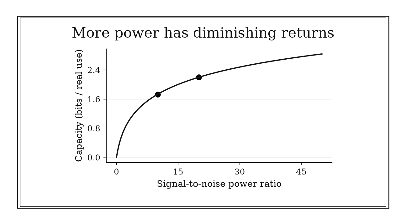
Figure 15.2. For a real scalar Gaussian channel, capacity is 0.5 log2(1+SNR) bits per use. Raising linear SNR from 10 to 20 adds about 0.47 bit, rather than doubling capacity.
15.3.3: Binary Symmetric Channel Capacity
History
A message can arrive perfectly intact even though every bit along the way had a real chance of flipping, and that outcome is the consequence Shannon proved possible in 1948. He modeled discrete noisy channels by transition probabilities and proved the noisy-channel coding theorem, and a channel that independently flips each binary symbol with probability (q) became the simplest lasting example, a direct specialization of that theorem. Individual bits stay unreliable no matter what; Shannon’s result was that sufficiently long, well-designed codes can still make the whole message arbitrarily reliable, at any rate below a fixed ceiling.
The equation
For a binary symmetric channel with independent flip probability (q),
where
A uniform input attains capacity.
How to read it
For a binary symmetric channel, capacity is (C=1-H_2(q)) bits per use, where (H_2(q)) is the binary entropy, the average bits of uncertainty the flip probability (q) creates. A uniform input makes the output carry a full bit of entropy; subtracting the flip’s own uncertainty leaves the useful information delivered. Capacity is a full bit at (q=0), falls to zero at (q=1/2), a channel conveying nothing, and rises again past (q=1/2) since a biased flip can be inverted at the receiver. Reaching capacity requires redundancy, extra structure beyond the raw message, across many uses.
How to use it
A satellite-link engineer models the downlink as a binary symmetric channel with flip probability (q=0.10) and needs the ceiling on reliable throughput. Binary entropy is (H_2(0.10)), so capacity is (C-0.469=0.531) useful bit per transmitted bit. Across (1{,}000) bits, the ceiling is about (531) information bits before finite-block penalties. The engineer treats (0.531) as the target for a well-designed long code, not a short uncoded stream. If the channel has burst errors clustering flips together rather than striking independently, this ceiling no longer applies and a different model is needed. This is an Independent rule: the flip probability directly determines the fundamental capacity of the idealized symmetric binary channel.
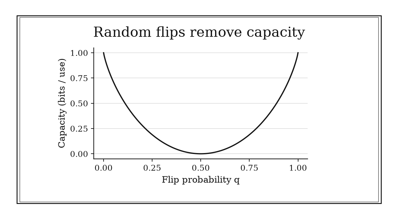
Figure 15.3. A binary symmetric channel has capacity 1-H2(q). Capacity vanishes at q=0.5 but recovers above one-half because a known tendency to flip can be inverted.
15.3.4: Optimal Prefix Coding Is Within One Bit of Entropy
History
Before 1951, nobody had proven which binary code was truly the best a fixed set of symbol probabilities could support; existing schemes worked well without a proof of optimality. Graduate student David Huffman, at MIT, was given a choice between sitting a final exam and writing a term paper on efficient binary coding, and he chose the paper. His bottom-up construction, repeatedly merging the two least likely symbols into one, produced the actual optimum among binary prefix codes, published in 1952. Huffman’s result did not say how close that optimum sits to the ideal average code length; the bracket below states that gap.
The equation
For a finite discrete source with base-2 entropy (H(X)), let (L^*) be the minimum expected length among binary prefix codes. Then
Ideal real-valued lengths are
Shannon lengths (-_2p_i) satisfy the Kraft inequality and establish the upper bound.
How to read it
Entropy (H(X)), the average bits of surprise per symbol, is a hard floor: no uniquely decodable code beats it on average. Rounding each symbol’s ideal length, (-_2p_i), up to the next whole number costs less than one extra bit per symbol, so an achievable prefix code lands within that gap: (H(X)L^*<H(X)+1). Huffman’s construction only improves on that rounded scheme; it cannot do worse.
How to use it
An archiver developer has measured a file format’s symbol entropy at (H=3.2) bits per symbol and wants to know what a Huffman tree can promise before building one. The bracket gives (3.2L^*<4.2) bits per symbol, never below entropy and never at or above (4.2). If the built tree averages (3.9) bits per symbol, the developer knows roughly (0.7) bit of the gap is rounding overhead, not a flaw in the algorithm, and reaches for arithmetic coding, which pushes closer to (3.2), only if the added complexity is worth that last fraction. The bracket assumes known, stable symbol probabilities; a coder sending header tables or handling correlated symbols spends real bits beyond this estimate. This is an Independent rule: entropy directly brackets the best average prefix-code length across lossless source-coding applications.
15.3.5: Bloom Filter Optimal Hash Count
History
Storing every item in a set exactly, with no possibility of error, can cost more memory than a system can spare, especially when most queries ask about items never inserted at all. In 1970, Burton H. Bloom proposed a compact hashed structure trading that certainty for space: it could answer “possibly present” for an item never inserted, a false positive, but under the basic insertion-only model it never answered “absent” for one that genuinely was. That controlled, one-sided error bought a large memory saving over exact storage. The hash-function count became the structure’s central tuning question.
The equation
For (m) bits, (n) inserted items, and (k) approximately independent uniform hashes, the false-positive rate is
It is minimized near
At that point,
How to read it
For (m) bits, the array’s storage slots, each 0 or 1, holding (n) inserted items and (k) hash functions, the false-positive rate is approximately (p_{}(1-e{-kn/m})k). After all insertions, any single bit is still zero with probability about (e^{-kn/m}); at the optimal hash count (k^*=(m/n)), that probability is exactly one half. Fewer hashes than the optimum leave bits unused; more hashes set nearly every queried bit to one, drowning the array in false matches.
How to use it
An airport baggage system logs scanned tag codes in a Bloom filter to catch duplicate scans without a full database, budgeted at (m/n=10) bits per expected tag. The optimal hash count is (k^*=10), rounding to seven, giving false-positive rate (0.6185^{10}), under one percent, about one in 122 new tags wrongly flagged and routed to a manual check. If the yard later handles more bags without resizing, (n) rises, (m/n) falls, and the false-positive rate climbs past budget. The system also assumes tags are only inserted, never deleted; clearing a bit to remove one could wrongly clear another’s evidence, a false negative the basic filter should not have. This is a Specialized rule: it tunes a particular probabilistic data structure after its memory budget, capacity, and acceptable error have been chosen.
Chapter Synthesis: Information Is Model-Relative but Not Metaphorical
Information theory begins by assigning a logarithmic cost to probability. Surprisal makes independent rarities additive. Entropy averages that cost and cannot exceed the log of a finite alphabet. Rare Bernoulli entropy shows that a dramatic event can carry many bits when it occurs but little average uncertainty across trials. Perplexity exponentiates predictive cross-entropy into an effective branching factor.
Dependence and processing then become measurable. Mutual information detects departures from independence that correlation can miss. Data processing limits every downstream representation that receives no side information. Pinsker converts a KL guarantee into a uniform bound on event probabilities.
Operational theorems complete the chapter. Gaussian distributions maximize differential entropy at fixed variance. Gaussian and binary-channel capacities set reliable-rate ceilings. Entropy brackets the best prefix-code length, while a Bloom filter chooses a deliberate one-sided error to save memory.
Across all twelve rules, ask four questions:
- Which probability distribution, alphabet, conditioning set, and log base define the quantity?
- Is the object pointwise surprisal, an average entropy, a dependence measure, or an operational capacity?
- Does a transformation receive side information, or is it limited by data processing?
- Is the result a universal limit under the model or a specialized design approximation?
One-Page Information Theory Toolkit
| Recognition cue | Rule to try | What it gives | Role |
|---|---|---|---|
| An event probability must become an additive score | Compute (-_2p) | Surprisal in bits | Independent |
| A finite alphabet bounds uncertainty | Use (H_2M) | Entropy ceiling | Independent |
| A binary event is very rare | Use (p_2(e/p)) | Rare-event entropy estimate | Independent |
| Average predictive log loss feels abstract | Exponentiate cross-entropy | Perplexity | Independent |
| Dependence may be nonlinear | Compute mutual information | General dependence measure | Independent |
| A representation is processed without new evidence | Apply data processing | Information-retention ceiling | Independent |
| KL divergence is small | Apply Pinsker | Worst event-probability error | Independent |
| Only variance is fixed | Compare with a Gaussian | Differential-entropy ceiling | Independent |
| A Gaussian channel has known SNR | Use log-one-plus-SNR | Capacity limit | Independent |
| A bit channel flips independently | Use (1-H_2(q)) | Binary-channel capacity | Independent |
| Lossless prefix compression is planned | Bracket length by (H) and (H+1) | Coding target | Independent |
| A Bloom filter has a bit budget and item count | Choose (k(m/n)) | Hash count and error estimate | Specialized |
Decision Path
- Is the question about one outcome? Use surprisal. If it asks for the average over a source, use entropy or cross-entropy instead.
- Is the alphabet finite? Apply the log-alphabet ceiling before accepting a larger uncertainty or mutual-information claim.
- Is a Bernoulli event rare? Use the small-(p) entropy approximation only after checking the regime and whether temporal dependence changes the entropy rate.
- Are predictive models being compared? Keep the tokenization, evaluation data, conditioning information, and log base fixed before comparing perplexity.
- Is dependence the target? Mutual information is broader than correlation, but finite-sample estimation and causal interpretation remain separate issues.
- Has information passed through a transformation? Draw the Markov diagram and identify any side information before invoking data processing.
- Must an information discrepancy become an event error? State the KL direction and units, then use Pinsker.
- Is the question operational? Match the exact source, channel, code, or probabilistic-data-structure assumptions before using the corresponding limit or tuning formula.
Transfer Problems
1. Move between probability, entropy, and perplexity
An outcome has modeled probability (1/64). Compute its surprisal. Then consider a predictor with cross-entropy (6) bits per token and translate that into perplexity. Explain why the two numerical values answer different questions even though both use logarithms.
2. Detect dependence and track processing loss
Let (X) be a fair sign taking values ({-1,1}), let (Y=X), and let (Z) discard the sign by reporting (Y^2). Compute or reason about (I(X;Y)) and (I(X;Z)), then identify the Markov chain that makes the loss unavoidable.
3. Separate a universal limit from a design choice
For a binary symmetric channel with flip probability (0.1), compute its capacity scale. Separately, size the hash count of a Bloom filter with (m/n=12) bits per item. State which result is a channel limit and which is an approximate implementation tuning rule.
Where These Ideas Reappear
- Probability: surprisal, entropy, KL divergence, and concentration all begin with a probability model and transform multiplicative likelihood into additive scale.
- Statistics and machine learning: cross-entropy is a proper scoring rule, mutual information measures dependence, and data processing limits feature representations.
- Combinatorics: log counts become information, while prefix trees and Bloom filters turn counting structure into algorithms.
- Asymptotics: rare-event entropy and coding limits use logarithmic expansions and large-block behavior.
- Signal processing and control: channel capacity, SNR, and data processing bound what sensors, filters, and feedback systems can convey.
- Scientific computing: log-domain arithmetic prevents underflow in likelihoods, while information inequalities quantify approximation loss.
- Computer systems: compression and probabilistic membership structures trade storage, computation, and controlled error.
Historical Notes and Sources
All twelve profiles have verified historical connections. Repeated use of Shannon’s 1948 paper reflects the number of distinct operational ideas developed within one communication framework; later terminology and concise rule wording are identified as modern interpretations.
- Hartley, logarithmic information, and alphabet size: Hartley, “Transmission of Information”; Shannon’s probabilistic generalization.
- Shannon’s entropy, mutual information, processing framework, and channel limits: Shannon’s 1948 paper; IEEE REACH primary-source edition.
- Perplexity in speech recognition: Jelinek et al., 1977; Brown et al., 1992.
- The Schützenberger–Pinsker attribution: historical study of Schützenberger–Pinsker inequalities; Pinsker’s 1960 paper record.
- Huffman coding: Huffman’s 1952 paper; MAA history of the discovery.
- Bloom filters: Bloom’s 1970 paper; DBLP bibliographic record.
- Modern information-theory statements: Stanford EE 376A course notes; Jurafsky and Martin, Speech and Language Processing.