Chapter 16: Measurement and Uncertainty: Building Trustworthy Results
A scale can return the same answer to three decimal places and still be wrong. Repetition can make the mean steadier, a spreadsheet can carry fifteen digits, and a report can display a narrow interval, yet none of those things repairs an unrecognized calibration offset. Trust begins by separating what varies from what remains wrong in the same direction.
Measurement uncertainty is therefore not decorative “plus or minus” notation. It is an accounting system. Every relevant source is expressed on a common standard-uncertainty scale, passed through the measurement model, combined with its dependencies intact, and reported at a precision the evidence can support.
The fourteen rules in this chapter form three groups. The first distinguishes scatter, bias, evaluation method, and reporting precision. The second propagates small uncertainties through powers, products, and general differentiable models. The third restores covariance, converts bounds and coverage conventions, prioritizes improvements, and identifies when local linearization should yield to simulation.
The governing habit is: write the measurement model and uncertainty budget before deciding how many digits, or how much confidence, the result deserves.
16.1: Scatter, Bias, and Reporting Discipline
Repeated observations answer only some uncertainty questions. These rules separate random scatter from common offset, distinguish how uncertainty was evaluated from how important it is, and keep numerical presentation from outrunning the evidence.
16.1.1: Repetition reduces random scatter, not fixed bias
History
Averaging away a bad reading tempts anyone patient enough to repeat it, yet a shared offset survives every repeat exactly as it started. In 1977 the International Committee for Weights and Measures asked the Bureau International des Poids et Mesures to settle disagreement among national laboratories over expressing measurement uncertainty. A questionnaire to 32 laboratories drew 21 replies, which an ISO working group turned into the 1993 Guide to the Expression of Uncertainty in Measurement, corrected in 1995.
The replies forced a distinction repetition cannot dissolve: repeated readings expose scatter around whatever center the instrument reads, while a calibration record shows whether that center is right.
The equation
Write one observation as
For independent errors,
The random term shrinks with (n); the fixed bias (b) does not.
How to read it
Write one reading as a target value plus a fixed offset, a systematic error pushing every reading the same direction, plus a wobble that differs by chance, a random error written (_i). Averaging (n) readings shrinks the wobble by (n), the way pooling many opinions tightens a poll’s margin, but the offset rides along unchanged, so the average inherits it exactly. A narrow spread among repeats measures only repeatability; it cannot confirm whether the reading’s center is right.
How to use it
A small-batch coffee roastery weighs green beans on a scale that a bench audit, checking it against a certified reference weight, shows reads (2.0) g high, with random standard deviation (1.0) g. The technician wants to know whether averaging a hundred weighings will fix the discrepancy before the next shipment ships.
With (n=100), the standard deviation of the mean falls to (1.0/=1.0/10=0.10) g, but the expected offset stays at (2.0) g in every average. If the offset instead drifted with the hopper’s fill level rather than staying fixed, treating it as one constant correction would leave a new, unbudgeted error. The technician sends the scale for calibration instead of scheduling more weighings. This rule directly answers whether more repeats can solve the observed problem. Independent.
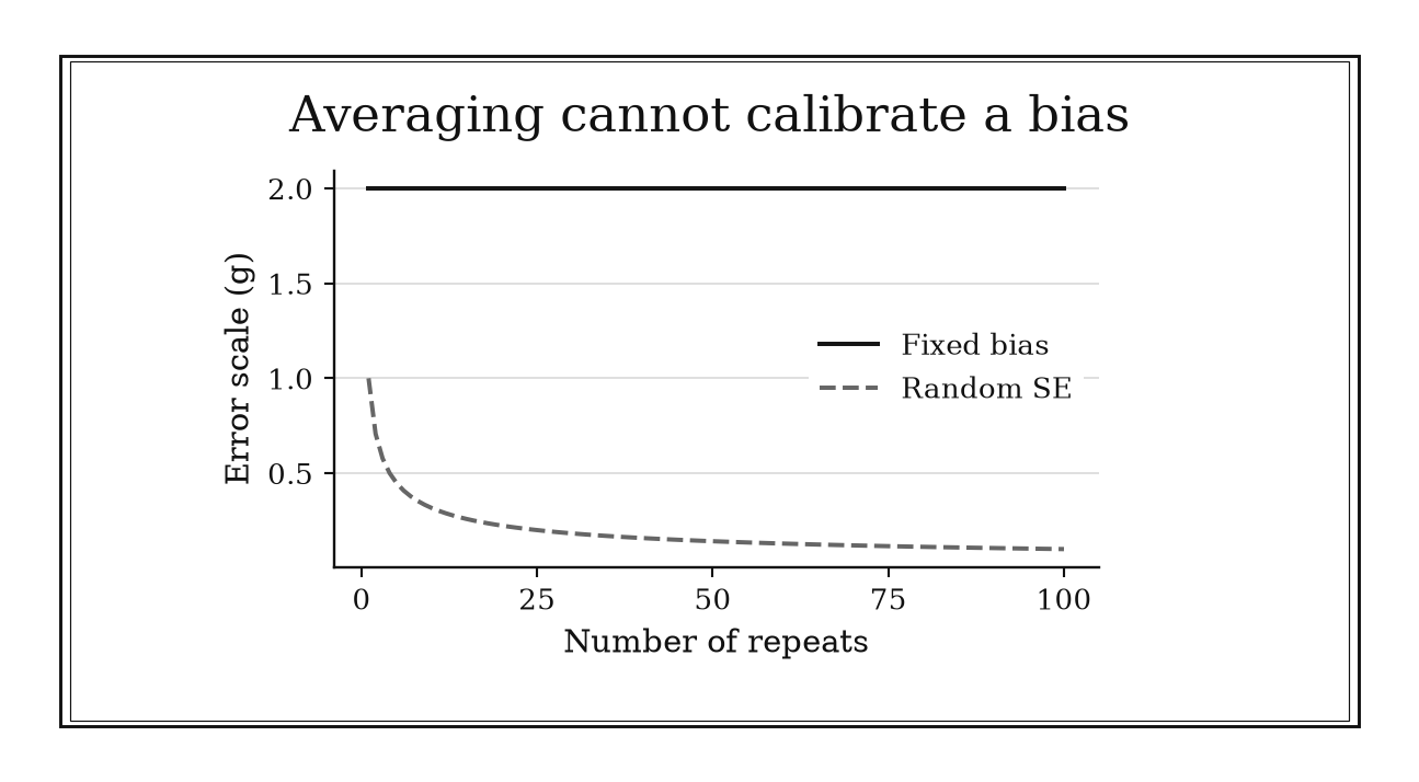
Figure 16.1. With fixed bias 2 g and single-reading SD 1 g, random SE shrinks as 1/sqrt(n) but bias stays at 2 g. More repeats improve repeatability without correcting the offset.
16.1.2: Type A and Type B describe evaluation methods, not importance
History
Whichever number enters an uncertainty budget can change whether a part passes inspection. After the 1977 CIPM request, BIPM’s questionnaire went out; 21 of the 32 laboratories answered, and the replies shaped the working group’s choice to classify every uncertainty component by its method of evaluation. Type A uses statistical analysis of repeated observations; Type B uses other information, such as calibration certificates or scientific judgment.
The categories were never stand-ins for random and systematic, or a ranking of rigor. Both convert to the same standard-uncertainty scale.
The equation
For (y=f(x_1,,x_m)), a first-order budget has the form
Nothing in this equation changes according to whether (u_i) came from a Type A or Type B evaluation.
How to read it
Type records the route by which a number was obtained, not how much it matters. Type A means the value came from statistics on repeated readings; Type B means it came from something else, such as a calibration certificate, a lab’s documented comparison of an instrument against a reference standard. Importance is decided afterward, by how much that input moves the result once scaled by its sensitivity. An old Type B certificate can dominate a budget built mostly from fresh readings, the way one trusted account can outweigh a dozen hurried glances.
How to use it
A machine shop measures a shaft’s diameter before shipping a batch of housings. Ten repeated gauge readings give repeatability uncertainty (u_A=0.020) mm, and the gauge’s calibration certificate lists (u_B=0.050) mm. With unit sensitivity and no shared cause, the combined contribution is
The certificate-based term dominates even though it came from no reading taken that day, so the inspector cannot dismiss it. If thermal expansion affects both inputs, the inspector checks whether one contribution was entered twice or distinct inputs are correlated. Duplicate entries must be removed; correlated inputs require covariance terms, whose effect depends on the sensitivity signs. This rule organizes a reusable budgeting procedure. Workflow.
16.1.3: Keep guard digits until the final reported result
History
Should a calculation carry extra digits it plans to discard, or round cleanly at every step? The GUM and NIST reporting framework, drawn from the 1993 Guide to the Expression of Uncertainty in Measurement and its 1995 corrected reprint, separates internal calculation from final expression: components are combined before the result and its expanded uncertainty are rounded for communication. That sequence guards against an old, quiet error: rounding at every step need not equal rounding once at the end.
The standards did not invent guard digits, but the reporting workflow they built gives the practice a documented place.
The equation
In general,
Under round-to-nearest with halves rounded upward,
How to read it
Each early rounding replaces a value with the nearest point on a coarser grid, and later arithmetic operates on that replacement instead of the real number, the way trimming a recipe’s measurements to the nearest teaspoon at every step, rather than once at the end, can leave a dish over- or under-salted. Carrying extra stored digits, guard digits, protects the arithmetic; it does not certify the measurement itself is known to that many places. RSS, root sum of squares, meaning squaring each contributor, adding, and taking the square root, is especially sensitive to early rounding.
How to use it
A small winery blends three tank samples to certify the alcohol-by-volume uncertainty on a shipment’s label. The three contributing uncertainties are (0.146), (0.154), and (0.155) percentage points. Combined by RSS on the unrounded figures,
Rounding each contributor first, to (0.1), (0.2), and (0.2), instead gives (==0.3000), a materially larger figure that could push the label into a stricter regulatory tier than the wine occupies. The winery keeps every intermediate value at full precision and rounds only the certified result, so the display rounding never becomes the calculating rounding. This rule belongs to the reporting workflow. Workflow.
16.1.4: Round the uncertainty first, then align the result
History
A result reported to five decimal places can imply a precision the measurement never earned. NIST Technical Note 1297, the United States implementation of the international Guide to the Expression of Uncertainty in Measurement, gives an explicit answer: state expanded uncertainty to at most two significant digits, then round the result to that same decimal position.
What it fixed was the order of operations; the digit count itself can vary by field. Settle the uncertainty’s reporting scale first, then stop the estimate from displaying resolution its uncertainty cannot support.
The equation
A typical transformation is
If two uncertainty significant digits are retained,
How to read it
The uncertainty decides how many decimal places the result may keep. Once that position is fixed by rounding the uncertainty, digits in the estimate further right imply a discrimination the budget does not back up, the way a receipt listing a total of (19.997) dollars makes no sense beside a payment rounded to the nearest cent. Nothing about the stored, unrounded values changes; only the reported pair is affected. Expanded uncertainty means the standard uncertainty scaled up by a coverage multiplier to state a wider band, not a raw measurement error.
How to use it
An electrician measuring line voltage during a compliance test computes (83.2746) V with expanded uncertainty (1.36) V from the meter’s specification sheet. The site convention calls for two significant digits in the uncertainty, so (1.36) rounds to (1.4) V.
The result rounds to match: (83.2746) becomes (83.3) V, giving (83.3) V rather than (83.2746) V, which would falsely suggest four-decimal confidence. Leaving the raw figure beside the rounded uncertainty would let an inspector read confidence the budget never supported. The electrician keeps the unrounded pair in the test log and reports only the aligned figures. This is a final reporting step, not a way to alter the underlying estimate. Workflow.
16.1.5: Mean-squared error is variance plus squared bias
History
A single scoring result, presented at the Fourth Berkeley Symposium in 1960, forced statisticians to reconsider what “accurate” meant. William James and Charles Stein showed that in the spherical multivariate-normal model with known common variance, an estimator that deliberately shrank every coordinate toward the origin could beat the ordinary coordinate-by-coordinate estimator under squared-error loss, for mean vectors with three or more coordinates. The paper appeared in the 1961 proceedings.
Shrinkage traded a deliberate bias for a larger variance reduction, illustrating the bias-variance identity below without being its origin.
The equation
For an estimator () with finite second moment,
where (()=E()-).
How to read it
Split the gap between an estimate and the truth into two pieces: its random deviation from its own average, and how far that average sits from the truth, its bias, a systematic offset in one direction. Squaring and averaging gives variance plus squared bias and removes the cross term, since the centered random part has expectation zero, the way a bakery deliberately overfilling every bag accepts a fixed bias to shrink underweight complaints. A method with zero bias is not automatically best. The identity cannot reveal bias from repeated measurements alone; that takes knowing the true target.
How to use it
A school district’s psychometrician is choosing how to report a small classroom’s average test score. The raw average is unbiased but noisy, with standard deviation (4), giving mean-squared error (4^2=16). A shrinkage method pulling the average toward the district mean introduces bias (1) but cuts the standard deviation to (3), giving
Under squared-error accounting the shrunken score wins, so the psychometrician recommends it for the file. Under a cost structure penalizing any deviation from a school’s own raw number, the bias term alone could matter more, so the psychometrician verifies that squared-error loss is the district’s actual criterion before filing the recommendation. This is a portable comparison rule once the target and loss are stated. Independent.
16.2: Propagation Rules and Their Assumptions
An output inherits uncertainty through its mathematical dependence on its inputs. These four rules move from a quick power-law estimate to a complete first-order budget, while making the small-uncertainty and independence assumptions visible.
16.2.1: A power multiplies relative uncertainty by its exponent
History
A small measurement error, run through a power-law shortcut with the wrong exponent, can turn into a badly understated volume, weight, or dose. The 1993 Guide to the Expression of Uncertainty in Measurement, product of the 1977 CIPM request and the ISO working group that followed, formalized propagation through sensitivity coefficients, derivatives converting an input’s uncertainty into output units. Applied to a power (y=Kx^a), that law gives a portable check: the exponent multiplies relative uncertainty, a modern specialization rather than the working group’s own phrasing.
The equation
For a smooth real branch of (y=Kx^a), typically with (x>0), and with (K), (y), and small uncertainty,
Equivalently, logarithmic differentiation gives
How to read it
Relative uncertainty means uncertainty expressed as a fraction of the measured value, so a distance known to within (1%) has relative uncertainty (0.01). The exponent (a) is a dimensionless sensitivity: a (1%) change in (x) produces roughly an (a%) change in (y), the way a small interest-rate error compounds over a long loan. Standard uncertainty uses (|a|) since a spread cannot be negative. A negative exponent flips the direction of change but not the size of the propagated uncertainty. The rule says nothing once relative uncertainty is large or the base sits near zero.
How to use it
A tank fabricator quotes the volume of a spherical propane tank, (V=(4/3)r^3), from a radius with relative standard uncertainty (0.8%). Since the exponent on (r) is (3), the contribution to volume uncertainty is
or on a nominal 5,000-gallon design, (0.024000=120) gallons flagged on the drawing.
For a fitting on an inverse-square flow relationship, a (2%) distance uncertainty instead contributes about (2(2%)=4%). The quoted (0.8%) is only trustworthy if the radius sits clear of the tank’s rolled-seam tolerance, where the true error can skew rather than stay symmetric, so the fabricator remeasures the seam before releasing the drawing. This rule directly converts one relative uncertainty into another. Independent.
16.2.2: Products and quotients combine relative uncertainties
History
A contractor who adds a (2%) error to a (3%) error expects (5%) slop in a material order; the real uncertainty of the computed area comes out smaller. The GUM’s first-order propagation law, built from the 1977 to 1995 international effort behind the 1993 Guide, propagates a measurement model through its derivatives and keeps covariance where inputs are dependent. Applied to a product of powers with uncorrelated inputs, it reduces to the familiar root-sum-of-squares rule for relative uncertainties, a calculation step derived from the framework, not a separate discovery.
The equation
For
with (K) and nonzero inputs on a smooth real branch, typically (x_i>0) for noninteger exponents, plus uncorrelated, modest relative uncertainties,
Covariance adds cross-terms when inputs are dependent.
How to read it
Taking logarithms turns multiplication and division into addition, so each factor’s relative uncertainty, its uncertainty as a fraction of its own value, contributes independently. Independent relative uncertainties combine the way independent wind gusts partially cancel more often than they align: by squaring each, adding, and taking a square root, not simple addition. A quotient needs no separate rule, since a denominator’s exponent is simply negative and squares positive regardless. The formula is silent about correlated inputs; correlation restores cross-terms it drops.
How to use it
A flooring contractor measures a room to price a hardwood job, finding length (L) with relative standard uncertainty (u_L/L=2%) and width (W) with (u_W/W=3%), independently measured with separate tape pulls. For area (A=LW),
or (3.61%). That is a relative standard uncertainty, not an ordering allowance. The contractor chooses an acceptable shortage risk and accounts for cutting waste before setting a material margin. If the same tape produced both readings, a stretch or calibration error would push length and width together, so the contractor measures with two tapes cross-checked against a reference length. This rule is a component of the uncertainty-propagation workflow. Workflow.
16.2.3: Scale every input uncertainty by its sensitivity coefficient
History
Before laboratories agreed on sensitivity coefficients, a raw input uncertainty in one unit had no reliable way to become a statement about an output in another unit. The ISO/BIPM working groups spent 1977 to 1995 building the GUM method, and sensitivity coefficients sit at its center. The measurement model is locally linearized, and each input’s standard uncertainty converts to output units through the measurand’s derivative with respect to that input.
The payoff was unit discipline: every component enters the budget in the measurand’s own units.
The equation
For (y=f(x_1,,x_m)), define
The derivative has units of output per unit input, so (c_i u(x_i)) has output units.
How to read it
The sensitivity coefficient answers one question: near the reported estimate, how much does the output move when this input moves by one unit? It is the model’s derivative there; multiplying it by that input’s standard uncertainty converts a raw uncertainty into output units. An input with tiny raw uncertainty can still dominate if the model is highly sensitive there, the way a small shift in a final drive gear can swing a machine’s output more than a larger shift elsewhere. The coefficient is a local slope and says nothing far from the operating point.
How to use it
A test engineer qualifies a cartridge heater whose power is (P=V^2/R), with fixed resistance (R=10) ohms and drive voltage (V=20.0) V measured with standard uncertainty (u(V)=0.1) V. The sensitivity coefficient is
on a nominal (P=20.0^2/10=40.0) W. Accepting the heater also requires a specified rating tolerance and an acceptance rule that accounts for uncertainty. Evaluating the derivative at the wrong operating point, say a supply sagging under load, produces a coefficient that no longer describes the real circuit, misstating the power uncertainty with no warning in the arithmetic itself. This coefficient is a reusable step inside a full budget. Workflow.
16.2.4: Build an uncertainty budget with sensitivity-scaled RSS terms
History
Add every input’s raw uncertainty for a worst-case bound, or combine them some other way that claims to be tighter? The 1977 CIPM questionnaire to 32 laboratories had gathered disparate uncertainty statements; the GUM turned them into one common variance budget. For uncorrelated inputs, its general law reduces to a root sum of squares of sensitivity-scaled standard uncertainties, settling the dispute for variance addition once independence is justified.
That reduction made each component auditable in the output’s own units, conditional on the model and independence assumptions.
The equation
For uncorrelated inputs,
It follows from the local approximation (y_i c_ix_i).
How to read it
Every input uncertainty is first translated into the output’s own units by its sensitivity coefficient, the way currency amounts convert to one currency before they can be added. Only after that translation do independent variance contributions add, with the final square root returning the total to the output’s scale. A list of raw uncertainties in mismatched units is not yet a budget. The formula assumes independent inputs, and it promises no coverage level.
How to use it
A fencing contractor sizes a gate opening (y=2L+W): a post setback (L) on each side plus a gate leaf width (W), with uncorrelated standard uncertainties (u(L)=0.10) mm and (u(W)=0.30) mm. The sensitivity coefficients are (2) and (1), so the combined standard uncertainty is
The contractor compares that uncertainty with the required gate tolerance using a stated coverage and acceptance rule. The uncertainty calculation alone does not set the tolerance. If the post setbacks and leaf width were cut from the same jig, a shared cutting error would correlate the two, understating the true uncertainty, so the contractor specifies separate cutting setups in the order. This is a full calculation workflow, not a stand-alone guarantee of coverage. Workflow.
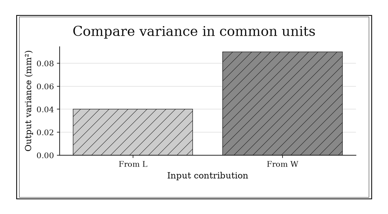
Figure 16.2. For y=2L+W with u(L)=0.10 mm and u(W)=0.30 mm, variance contributions are 0.04 and 0.09 mm². Their sum gives combined standard uncertainty sqrt(0.13)=0.361 mm.
16.3: Dependence, Coverage, and Escalation
The shortest uncertainty formulas are safe only under their assumptions. These rules restore correlation, turn bounded information into a standard deviation, distinguish standard from expanded uncertainty, target improvement effort, and identify when simulation is warranted.
16.3.1: Keep covariance terms for correlated uncertainties
History
Two measurements sharing the same reference standard rarely make their errors cancel the way independence would predict. Between 1977 and 1995 the CIPM and ISO/BIPM working groups wrote the international Guide to the Expression of Uncertainty in Measurement. It never assumed every input was independent. Its general propagation law explicitly retained covariance terms, which matters whenever quantities share a calibration, reference, environment, or processing step.
The modern rule warns against quoting only the simplified root-sum-of-squares special case. Dependence was part of the documented standard from the outset, not a later patch.
The equation
For a first-order model,
Using ((X_i,X_j)=_{ij}u_i u_j) makes the correlation explicit.
How to read it
Covariance is a number describing whether two inputs’ errors tend to move together, positive correlation, or in opposite directions, negative correlation, the way two singers following one off-key radio drift together while soloists drift apart. Whether that increases or decreases the output’s uncertainty depends on both the correlation’s sign and the sensitivity signs involved. Shared movement can cancel inside a difference and reinforce inside a sum. The formula does not supply the correlation value; that number must be justified rather than guessed.
How to use it
A clinical laboratory reports the difference between two correlated assay results from the same patient sample, (y=x_1-x_2), where both share the same instrument calibration and equal standard uncertainty (u) with correlation (). If (u=1),
not the (=1.414) an independence assumption would report. Treating the readings as independent would overstate the difference’s uncertainty by more than double, potentially making a real change harder to distinguish from measurement noise. For the sum of the same readings, the positive correlation would instead increase the combined uncertainty. The lab traces the shared calibration to justify the (0.8) before reporting either combination. Keeping covariance is a required budgeting step. Workflow.
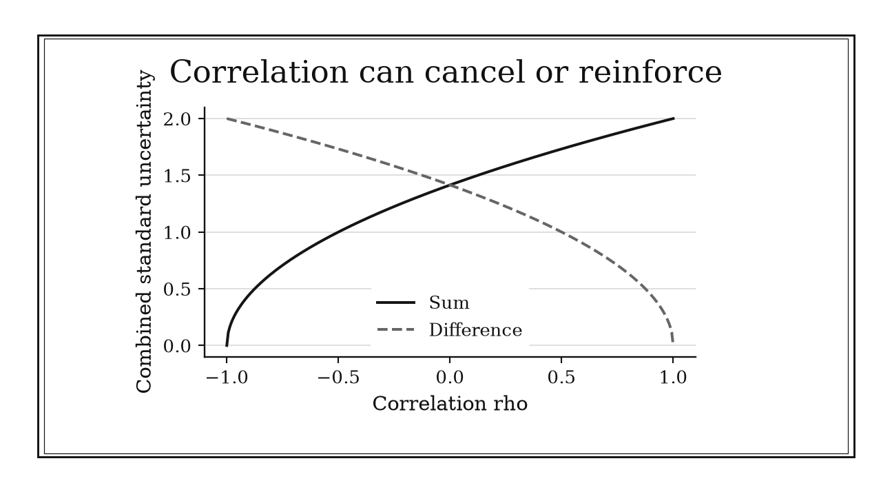
Figure 16.3. For two inputs with unit standard uncertainty, positive correlation raises uncertainty of their sum but lowers uncertainty of their difference. The sensitivity signs determine the effect.
16.3.2: Convert a uniform half-width to standard uncertainty with
History
A tolerance printed on a specification sheet looks like a hard boundary, not a probability statement, yet a laboratory has to turn it into one anyway. The GUM and NIST guidance address exactly this kind of input, one known only through symmetric bounds; the treatment dates to the 1977 to 1995 standardization push. When every value in an interval is judged equally plausible, the guidance models it with a rectangular distribution and converts its half-width into a standard uncertainty.
The division models incomplete knowledge: the spec bound is treated as equally likely everywhere inside its limits.
The equation
If the error (X) is uniform on ([-a,a]), then
Here (a) is the half-width, not the full interval width. Using the full width in the numerator would double the resulting standard uncertainty.
How to read it
Standard uncertainty is a standard deviation, so a hard bound cannot simply be typed in as though it already were one. The divisor () comes from integrating squared deviations across an equally weighted interval, the way a dart equally likely to land anywhere in a band spreads differently than one clustering near the bullseye. Here (a) is the half-width, center to edge; using the full width doubles the result by mistake. The rectangular model is a choice; the rule cannot reveal the error’s true distribution.
How to use it
A grain elevator’s truck scale displays weight rounded to the nearest (0.1) kg, so rounding error on any reading is bounded by (a=0.05) kg, with no value inside that band favored. Under the rectangular model,
An elevator operator adds that figure into the shipment’s declared-weight budget instead of treating the rounding as zero. If evidence favors values near the center, the operator reassesses the distribution. A symmetric triangular model on the same bounds gives (a/), but requires support beyond symmetric rounding alone. The operator checks the rounding rule and evidence about where unrounded readings fall within each display step. Selecting and documenting the distribution is part of the workflow. Workflow.
16.3.3: Coverage factor two is an approximate 95% convention
History
A laboratory reporting only a bare plus-or-minus figure leaves a regulator, patient, or court no way to know how much confidence that number carries. The GUM distinguishes combined standard uncertainty from expanded uncertainty and describes multiplying the combined figure by a coverage factor, a multiplier widening it into a stated interval. NIST’s 1994 implementation identifies (k=2) as the convention giving approximately 95 percent coverage under a normal approximation.
The qualification matters: the standards required the factor and the intended coverage stated alongside every expanded uncertainty; two standard deviations alone do not guarantee 95 percent coverage.
The equation
For a standard normal variable (ZN(0,1)),
Small effective degrees of freedom may call for a Student-(t) factor larger than two.
How to read it
Combined standard uncertainty is the single standard-deviation-scale figure left after every input’s contribution is converted to output units and combined. A coverage factor is the multiplier applied to widen that figure into a stated interval, the way saying a bus “usually” arrives within ten minutes means little without stating how often “usually” holds. Real coverage depends on the distribution’s shape and whether the interval was built the way the convention assumes.
How to use it
A pharmaceutical analytical lab certifies the mass of an active ingredient, with combined standard uncertainty (u_c=0.35) mg from its propagation budget. Applying (k=2) gives
so the certificate states (y) mg, expanded uncertainty with (k=2), approximately 95 percent coverage under the stated approximation.
A regulator judging whether a dose falls within its approved range needs the stated (k) and coverage claim alongside the bare (0.70) mg. If a boundary near zero makes the output strongly skewed, the lab checks coverage using an appropriate output-distribution model. Low effective degrees of freedom are a separate issue: a larger Student-t factor can be appropriate when the assumptions behind that approximation hold. This is a reporting convention embedded in an uncertainty workflow. Workflow.
16.3.4: Improve the dominant uncertainty contributors first
History
Polishing the easiest measurement to improve, rather than the one that dominates the final number, wastes a laboratory’s calibration budget without shrinking its uncertainty by much. The GUM process that emerged between 1977 and 1995 makes every sensitivity-scaled component visible in one budget. Once every contribution shares output units, variance shares show where effort can actually matter.
The framework established the budget; ranking components by propagated variance is a modern use of it, not a rule the delegates wrote.
The equation
For uncorrelated inputs,
The (q_i) are fractional variance contributions, not fractional standard-deviation contributions.
How to read it
Because variances add rather than the underlying standard uncertainties, shrinking a small term barely moves the combined total, the way fixing a leaky faucet does less for a water bill than fixing a burst pipe, even if the faucet is easier to reach. A single input can dominate through a large raw uncertainty, a large sensitivity coefficient, or both. Ranking raw sensor specifications alone, without scaling by sensitivity, can send effort toward a component that only looks large in its own units. The ranking leaves out cost, safety, and feasibility, and the shares must be recomputed after any upgrade.
How to use it
A municipal water utility’s metering program has three uncertainty contributions in its flow-measurement budget, worth (4), (1), and (1) variance units after scaling. The first supplies
two-thirds of the total variance. Eliminating either small term reduces the combined uncertainty only from (=2.45) to (=2.24). Halving the dominant term’s standard uncertainty instead changes its variance from (4) to (1), cutting the total to (=1.73), a far larger gain. Chasing the small contributors first because their parts are cheaper spends the budget for a fraction of the gain. The utility recalculates after the upgrade, since removing the dominant term can expose a new limiting factor. Prioritization is a workflow decision, not a universal property of the instrument. Workflow.
16.3.5: Use Monte Carlo propagation when linear uncertainty rules bend
History
A symmetric uncertainty estimate can quietly claim territory the real answer can never reach, unnoticed until the model is pushed hard enough to expose it. First-order propagation became the international default with the 1993 GUM. In 2008 the Joint Committee for Guides in Metrology issued Supplement 1 for cases where nonlinear models make linearization unreliable, describing how to sample the input model, pass the draws through the measurement equation, and compare the result with the analytic GUM calculation, a standards-body extension that keeps the linear method as its reference point.
The equation
Draw jointly from the input model and evaluate the full measurement equation:
Estimate the output distribution, standard uncertainty, and coverage interval from the (y^{(s)}).
How to read it
Monte Carlo propagation means running the actual measurement equation many times on randomly drawn, plausible input values, then reading the standard uncertainty and coverage interval off the spread of the resulting outputs rather than off a single tangent-line approximation, the way tasting the whole pot beats judging a stew from one spoonful. It keeps curvature, hard bounds, and skew that a first-order approximation smooths away. It cannot repair a wrong measurement equation or an unjustified input distribution.
How to use it
An irrigation engineer computes an application rate (Y=1/X), where (X) is a flow-time measurement uniform on ([1.5,2.5]) minutes per unit volume. Its standard uncertainty is (u_X=1/=0.2887). Derivative propagation about (x=2) gives (u_Yu_X/2^2=0.2887/4=0.0722) around (0.5). These are a center and a standard uncertainty, not a guaranteed range or a specified coverage interval.
Monte Carlo simulation preserves the output’s bounded range, (0.4) to (0.6667), and estimates a coverage interval for a stated probability. Here the exact equal-tail 95 percent interval is ([1/2.475,1/1.525]); it provides a check on the simulation. A normal linearized 95 percent interval, (0.5(0.0722)), extends below the possible range and has a lower upper endpoint. The engineer chooses the coverage needed for the pump-sizing decision and runs enough draws to stabilize its tail estimate. Monte Carlo is a reusable escalation step within the uncertainty workflow. Workflow.
Chapter Synthesis
A trustworthy result begins with a model of how observations arise and how inputs combine. Replication reduces independent scatter but not common bias. Type A and Type B say how a component was evaluated, not whether it matters. Internally, calculations retain guard digits; externally, the uncertainty sets the justified reporting position.
First-order propagation then supplies a common language. Powers scale relative uncertainty by their exponents, products combine relative contributions, and general models translate each input through a sensitivity coefficient. Covariance must remain wherever inputs share causes. Bounds require a distributional interpretation, and (k=2) requires a coverage qualification.
The budget is also a decision tool. Variance shares identify the improvements with leverage. When curvature, bounds, skewness, or near-zero denominators defeat linearization, Monte Carlo propagates the fuller model, but only as honestly as its inputs permit.
One-Page Toolkit
| Question | Quick rule | Principal condition |
|---|---|---|
| Will more repeats remove the problem? | Random SD of a mean falls as (1/n); fixed bias remains | Independent zero-mean scatter and genuinely fixed bias |
| How should components be classified? | Type A = statistical evaluation; Type B = other information | Convert both to standard uncertainties without duplication |
| How should the result be rounded? | Round uncertainty first; align the result’s decimal place | Preserve unrounded internal values |
| What does a power do? | (u_y/ | y |
| How are independent products propagated? | RSS of exponent-weighted relative uncertainties | Nonzero, uncorrelated inputs |
| What is one input’s contribution? | (u_{y,i} | c_i |
| What if inputs correlate? | Keep (2c_ic_j_{ij}) | Justified covariance model |
| How does a rectangular bound become (u)? | (u=a/) | Uniform model on ([-a,a]) |
| Does (k=2) guarantee 95%? | No; it is an approximate normal convention | State factor, method, and intended coverage |
| What should be improved first? | Rank propagated variance shares (q_i) | Uncorrelated contributions; assess covariance and model effects separately |
| When should linear propagation stop? | Use Monte Carlo for strong curvature, bounds, or skewness | Defensible joint input distributions |
Decision Path
- Define the measurand and write (y=f(x_1,,x_m)), including corrections.
- List every uncertainty source and possible shared cause. Label its evaluation Type A or Type B without treating the label as a rank.
- Convert each source to a standard uncertainty, retaining its units, distribution, divisor, and evidence.
- Calculate sensitivity coefficients and covariance terms. Use relative shortcuts only when their assumptions match the model.
- Inspect variance contributions and improve the components with genuine leverage.
- Challenge the linear approximation with scale, curvature, bounds, and limiting cases. Switch to Monte Carlo if it bends.
- Choose a coverage convention, round the uncertainty first, align the result, and report enough method detail to reproduce the claim.
Transfer Problems
1. Repetition versus calibration
A thermometer’s reading is (0.60^) high, with independent random SD (0.40^). Compare the expected error and standard error after (n=4) and (n=100) repeats. Which part can more repetition reduce, and what intervention addresses the other part?
2. A correlated quotient
A calculated density is (=m/V). The relative standard uncertainties of mass and volume are 0.5% and 1.2%, and their correlation is 0.30. Derive the covariance-aware relative uncertainty, paying attention to the negative exponent of (V), and compare it with the independence result.
3. A nonlinear bounded input
An output is (Y=1/X), where (X) is bounded to ([0.8,1.2]) but its distribution is disputed. Explain how a uniform assumption, a triangular assumption, and direct Monte Carlo propagation would change the budget and what evidence you would request before reporting a 95% interval.
Where These Ideas Reappear
Bias–variance accounting returns in statistical estimation, machine learning, and regularization. Sensitivity coefficients are derivatives from calculus and condition estimates from numerical analysis. Root-sum-square propagation is the variance algebra used throughout probability, while covariance connects directly to portfolio analysis, generalized least squares, and correlated sensor fusion.
Dimensionless relative uncertainty anticipates elasticity and nondimensionalization in applied mathematics. Monte Carlo propagation connects this chapter to simulation, Bayesian posterior prediction, reliability, and risk analysis. The same discipline, state the model, retain dependencies, and escalate when the approximation bends, will govern every later computational chapter.
Historical Notes and Sources
The international consensus story and most measurement conventions in this chapter are documented in JCGM 100:2008, the official GUM text and historical foreword and NIST Technical Note 1297. The nonlinear escalation story comes from JCGM 101:2008, Supplement 1 on Monte Carlo propagation. The shrinkage episode is supported by James and Stein’s primary paper, “Estimation with Quadratic Loss”. These sources are the ones recorded in the matching local research and historical-story files; the compact rule wording and present-day applications are modern interpretations.