Chapter 17: Financial Mathematics: Comparing Money Across Time
A 50% loss followed by a 50% gain does not return an investment to where it began. One hundred dollars falls to fifty, then rises only to seventy-five. The percentages look symmetric; their bases are not. Much of financial mathematics exists to prevent that kind of silent mismatch.
Money comparisons require a timeline. Rates must use compatible periods and compounding conventions. Inflation and investment growth must be put on the same multiplicative basis. Cash flows at different dates must be moved to one valuation date before they can be added. Only then do shortcuts and closed forms become trustworthy. Financial accumulation and discount factors are assumed positive: each effective periodic rate exceeds (-100%), and each payment count is a positive integer. Zero-rate limits and any stricter convergence or growth conditions are stated where needed.
The twelve rules in this chapter move from portable mental arithmetic to full discounted-cash-flow reasoning. The final group recognizes geometric patterns, annuities, perpetuities, savings deposits, and amortizing loans, without losing track of payment timing.
These are valuation tools, not investment recommendations. Taxes, fees, default, liquidity, uncertain cash flows, and personal constraints can dominate a neat formula. The governing habit is: draw the timeline, normalize the rate, and value every amount at one date before comparing alternatives.
17.1: Portable Mental Arithmetic
Quick estimates are valuable when they expose scale and asymmetry. Their speed comes from assumptions, so each result should be treated as a screen and checked exactly when the decision is sensitive.
17.1.1: Rule of 72 for doubling time
History
Did Luca Pacioli invent the doubling shortcut, or merely write down something merchants already used? His Summa de arithmetica includes an early printed version of what is now called the Rule of 72: divide 72, a number divisible by nearly every common rate, by the annual rate to estimate years to double. The book proves the trick was in print by 1494; whether Pacioli devised it or copied a habit already common among merchants, the record does not say.
The equation
For a constant positive effective annual rate written as a percentage,
The exact doubling time is
where (r) is written as a decimal and periods match the rate.
How to read it
(T_2) is the number of years until an amount doubles, and (r_{%}) is the annual rate written as a whole number, such as 9 rather than 0.09. Dividing 72 by that number estimates (T_2) directly. Doubling time grows without bound as the rate falls toward zero: dropping from 3% to 2% adds twelve years, (72/3=24) to (72/2=36). The shortcut assumes one steady compounded rate; it cannot show a return swinging above and below that rate year to year.
How to use it
A warehouse supervisor, 45, has ($40{,}000) saved at a steady 8% a year and wants to know whether it can double before he turns 54, (54-45=9) years away. The shortcut gives (72/8=9) years, right on schedule; the exact value is
about two days off. He keeps contributing rather than chasing a faster fund. The catch is the word steady: his real annual returns will swing above and below 8%, and (72/8) says nothing about that swing, only about one constant compounded rate. A bad early year restarts the doubling clock from a smaller base; averaging good years against bad ones is not the same as compounding the sequence he lived through. This shortcut directly answers a portable growth question under a stated rate. Independent.
17.1.2: Real return is approximately nominal return minus inflation
History
A dollar can grow while what it buys shrinks. Irving Fisher named that trap in The Theory of Interest (1930), where he separated interest measured in money from interest measured in goods and worked out their multiplicative relationship to the price level. The familiar shortcut, subtract inflation from the nominal rate, compresses that exact relation into arithmetic simple enough for a kitchen table; it is a modern reading of his work, not his own phrasing.
The equation
If (r_n) is nominal return and () is inflation over the same period,
so
How to read it
(r_n) is the return an account statement shows, () is inflation over that stretch, and (r_{real}) is what the return is actually worth once rising prices are subtracted out. Money grows by (1+r_n) while prices grow by (1+); dividing one by the other, then subtracting 1, gives the true real rate, and plain subtraction is a shortcut for that ratio, accurate when both rates are modest. It does not tell you which prices count: a household’s own basket can run ahead of or behind a broad national index.
How to use it
A grain farmer holds this year’s crop-sale proceeds in an account paying 8%, while fertilizer and diesel prices have risen 3% over the same stretch. Subtracting gives an approximate real return of (8-3=5%). The exact figure is
or 4.85%, confirming that the cash gained ground against those input costs over the measured period. Holding the balance rather than prepaying next season’s inputs also requires a forward-looking comparison of expected account returns, input-price changes, and any prepayment discount. The shortcut also assumes the stated 8% is what he actually keeps; taxes reduce the return before any inflation adjustment, and a national price index would tell a different story than his own fuel and fertilizer costs. This rule directly converts a money return into a purchasing-power screen. Independent.
17.1.3: Loss recovery is mathematically asymmetric
History
Federal Reserve historians still cite one number: a fall of roughly 89 percent in the Dow Jones Industrial Average from its 1929 peak to its 1932 trough. Turning that drawdown into a lesson about recovery percentages is this book’s application. An 89 percent loss needs far more than an 89 percent gain to erase it; recovering from 11 percent of the old peak requires a gain of roughly 809 percent.
The equation
If a fraction (L), with (0<L<1), is lost, the required gain (G) on the remainder satisfies
Therefore
How to read it
(L) is the fraction lost and (G) is the fractional gain needed to get back to even. The two percentages measure from different bases: the loss is a fraction of the larger starting amount, the gain a fraction of the smaller amount left behind, so equal-looking percentages cannot cancel unless nothing was lost. As the loss nears 100%, the required gain grows without bound. This rule leaves the recovery timeline open; it fixes only how large the gain must be.
How to use it
A hardware store owner finds a flood ruined 40% of his inventory, leaving (100%-40%=60%) intact, and his adjuster proposes a restocking budget equal to 40% of the surviving inventory’s value. Rebuilding the surviving 60% to full value requires a gain of
or 66.7% of the surviving value, not 40% of that smaller base. This replacement amount is still 40% of the original inventory value. The owner requests financing for the missing inventory using that fixed base; a budget described only as “40% of value” is ambiguous until its denominator is named. If inventory prices change, the replacement-cost calculation also needs updating. This is pure portable percentage arithmetic once the common base is identified. Independent.
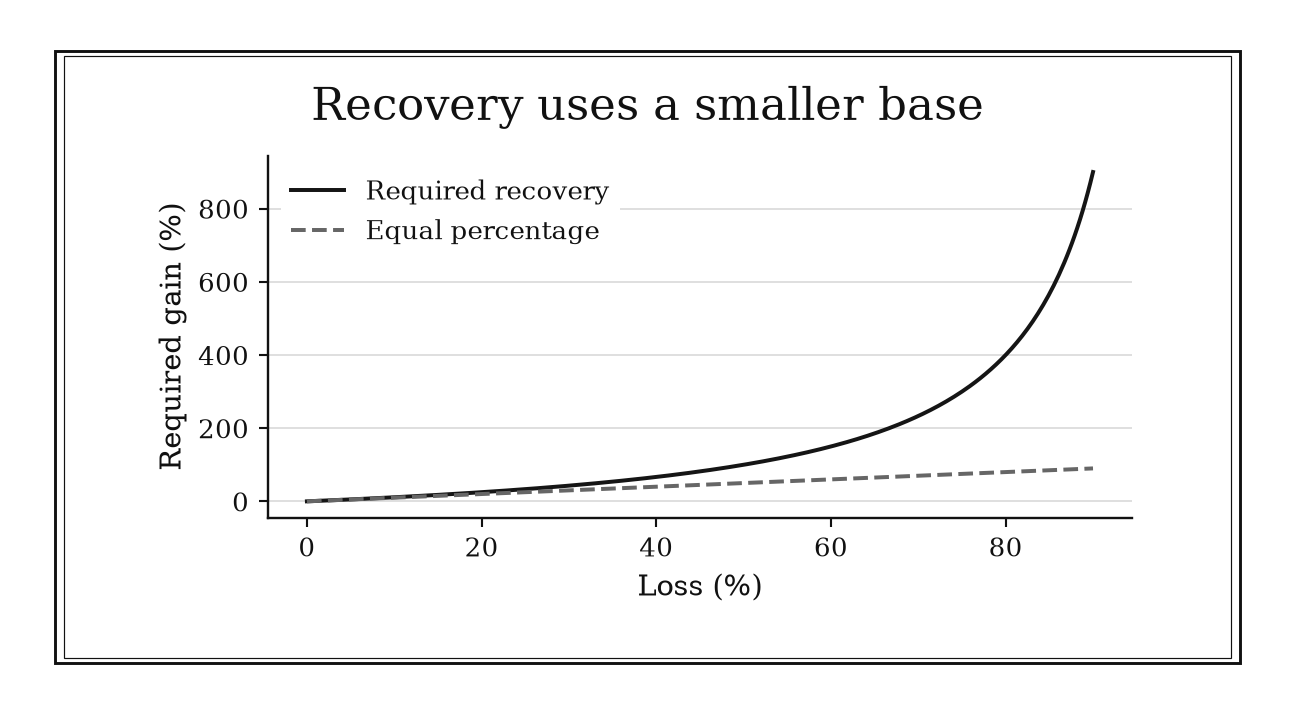
Figure 17.1. A loss L requires gain L/(1-L) on the remainder. A 40 percent loss requires about 66.7 percent recovery; equal loss and gain percentages do not cancel.
17.2: Put Rates and Cash Flows on One Basis
Quoted percentages and dated amounts are not directly comparable until their conventions match. These rules normalize compounding, move cash flows to one date, and turn the result into a basic project-value screen.
17.2.1: Convert periodic rates to an effective annual rate
History
Comparing two interest rates fairly used to be a matter of trust: a bank could quote a rate compounded monthly against a rival’s rate compounded daily. Congress addressed that with the 1991 Truth in Savings Act, and the Federal Reserve’s Regulation DD, effective 1992, working out of Washington, D.C., required every deposit account to disclose a standardized annual percentage yield, compounding a stated periodic rate onto a common one-year basis. It is a direct legal application of effective-rate logic, credited to no single regulator.
The equation
If (i) is the effective rate per compounding period and there are (m) periods per year,
For a nominal annual rate (j=mi),
How to read it
(i) is the interest rate credited each compounding period, such as each month, and (m) is how many periods fall in a year. Raising (1+i) to the power (m), then subtracting 1, gives the effective annual rate: the true one-year growth once each period’s interest earns its own interest. A nominal annual rate just multiplies (i) by (m), ignoring that compounding, so it understates the effective yield when the periodic rate is positive and (m) exceeds one. At a zero rate the two are equal. It ignores fees or a promotional rate that applies for only part of a term.
How to use it
A rural clinic’s business manager is comparing two equipment-financing quotes: one lender advertises 18% compounded monthly, meaning a monthly rate of (18%/12=1.5%); the other advertises 19% compounded annually. Multiplying the first rate by 12 makes it look cheaper, but the effective annual rate is
or 19.56%, higher than the second lender’s flat 19%, so she takes the second offer. Before signing, she checks whether either quote hides an origination fee, since the EAR formula converts compounding conventions but does not audit the rest of the contract. A loan’s APR can also follow a different disclosure convention than a deposit’s APY. This rule directly normalizes a fixed periodic compound rate. Independent.
17.2.2: Discount each future cash flow to the same date
History
A payment due today, added without adjustment to one due next year, overstates what a project is worth: a dollar in hand can earn a return before the later one arrives. In 1671 Johan de Witt built his valuation the opposite way, presenting the States of Holland with an analysis that combined survival probabilities with discounting to compare the government’s life annuities against redeemable bonds, valuing each dated payment on its own. His calculation carried the extra complication of mortality; the modern formula generalizes his core move of bringing every future amount to one valuation date first.
The equation
At a constant effective rate (r) per matching period, present value at time zero is
More generally, time-varying rates use the accumulated discount factor (_{s=1}^{t}(1+r_s)).
How to read it
(C_t) is the cash amount arriving at time (t), and (r) is the rate per period a dollar could otherwise earn. Dividing (C_t) by ((1+r)^t) answers a simple question: how much would you need today to grow into (C_t) by then? Once every payment is expressed that way, ordinary addition becomes meaningful again. What discounting cannot do is make risk vanish; a shaky promise and a safe one, discounted at the same rate, come out looking equally reliable, which they are not.
How to use it
A city clerk is comparing two ways a state grant could fund a park project: ($200{,}000) today, or ($105{,}000) today plus ($105{,}000) in one year. Added at face value the second option totals (105000+105000=$210{,}000), but at a 5% rate the city could otherwise earn, its present value is
Since ($205{,}000) exceeds the flat ($200{,}000) option, the clerk recommends the split payment. She still flags that the comparison assumes the second payment is as certain as the first; if it depends on a future vote, the safe 5% rate understates its true risk. This calculation is a prerequisite inside valuation rather than a complete decision by itself. Workflow.
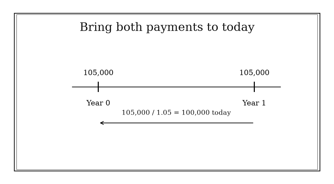
Figure 17.2. At an effective annual rate of five percent, 105,000 today plus 105,000 in one year has present value 205,000. Discounting aligns dates; it does not establish that the later payment is certain.
17.2.3: Positive NPV is the basic discounted-cash-flow screen
History
Treat every investment choice as a comparison of dated cash against a single opportunity-cost rate, and a workable accept-or-reject test falls out. That is the consequence Irving Fisher drew in his 1930 Theory of Interest: once income and cost streams are converted to present value at the going rate, an investment is worthwhile only when its dated benefits exceed its dated costs. The acronym NPV and today’s screen came later; Fisher supplied the framework.
The equation
With signed net cash flows (C_t),
For a conventional stand-alone project,
passes the basic discounted-cash-flow screen at rate (r).
How to read it
(C_t) is the net cash flow at time (t), outlays negative and receipts positive, and (r) is the opportunity-cost rate the money could otherwise earn. Adding every (C_t/(1+r)^t) collapses a dated schedule into one present-value number. A positive total means the modeled inflows outweigh the outlay and required return together; negative means they do not clear that bar. A positive NPV does not confirm the forecast is trustworthy; it only checks whether the numbers fed in clear the bar.
How to use it
A bakery owner is deciding whether to buy a ($1{,}000) walk-in cooler expected to save ($600) a year for two years, at a required 10% return. The net present value is
Since that result is positive, the purchase passes the screen and she buys the cooler. The margin is thin, built from one summer’s records; a slower year or a repair bill could erase it. She stress-tests the figure against a leaner estimate and checks whether financing changes the discount rate. NPV is a workflow gate whose credibility cannot exceed its forecasts and discount model. Workflow.
17.3: Recognize Repeating Cash-Flow Patterns
Level or steadily growing payment streams are geometric series. Recognizing the pattern saves arithmetic, but the closed form is valid only after payment count, timing, rate period, and growth convention have been pinned down.
17.3.1: Present value of an ordinary annuity
History
Johan de Witt told the States of Holland in 1671 that the government was selling its life annuities too cheaply. To make the case, he summed each dated, survival-weighted payment at its own discounted value rather than a flat rule of thumb. Strip away his mortality weighting and the calculation reduces to equal payments discounted period by period, the finite series behind this rule’s closed form. The compact formula packaging that sum into one factor is a modern specialization; adding discounted, dated payments is de Witt’s.
The equation
For (n) equal payments (C) made at the end of periods (1,,n), with effective rate (r) per period,
At (r=0), the limiting value is (nC).
How to read it
(C) is the level payment at the end of each period, (r) is the rate per period, and (n) is the number of payments. The formula compresses the finite sum (C/(1+r)++C/(1+r)^n) into one factor, worth as much today as a single lump sum. “Ordinary” means the first payment lands one period from now. What the formula will not catch is a miscounted schedule: pricing four payments as if there were five overstates the value, and nothing flags the error.
How to use it
A retired teacher is offered a pension buyout: a lump sum today instead of 5 more years of ($1{,}000) year-end payments. At a 6% rate she could reasonably earn, those payments are worth
today. If the buyout offer is ($4{,}500), she takes it, since it exceeds the annuity’s value; if the offer were ($3{,}900), she would keep the payments. She double-checks the payment count: if the stream actually runs 6 years, not 5, the value rises to
enough to flip which option wins. She also confirms the first payment truly starts a year out; an immediate first payment needs a different formula. This rule directly values a common finite pattern once its timing convention is established. Independent.
17.3.2: Constant perpetuity value is payment divided by rate
History
How do you put a price on an income stream that has no scheduled end? Britain faced exactly that problem in 1751, consolidating several existing debt issues into stock paying a fixed annual amount with no redemption date, securities that came to be called Consols. They supplied a real, long-lived example of a level payment continuing indefinitely, valued at whatever the market discount rate implied. The formula dividing the payment by that rate is a modern reconstruction, not a claim that eighteenth-century traders used this notation.
The equation
For a constant end-of-period payment (C) forever and constant effective rate (r>0),
It is the convergent series
How to read it
(C) is a level payment arriving at the end of every period, forever, and (r) is the discount rate, always greater than zero. Dividing (C) by (r) gives the present value of the infinite stream, because payments shrink fast enough, by (1/(1+r)) each period, to add to a finite total. Halving (r) doubles the value, since a smaller rate discounts distant payments more gently. The formula does not examine whether “forever” is realistic: it assumes the stream never ends and the rate never moves.
How to use it
A small town’s library board has just received a bequest and is deciding how much to treat as a permanent endowment versus spend on this year’s repairs. Setting aside ($200{,}000) to fund a ($10{,}000) annual acquisitions budget forever, at the 5% long-run return the board expects, implies an endowment value of
exactly matching the amount set aside, so the board treats the plan as funded. At a conservative 4% return instead, the same payment implies a required endowment of (10000/0.04=$250{,}000), a shortfall of (250000-200000=$50{,}000). The budget also may need to rise with costs, since a level nominal payment does not keep pace with rising book and journal prices. This rule directly prices an idealized constant stream under strict conditions. Independent.
17.3.3: Growing perpetuity value depends on the rate spread
History
A firm buying new equipment needs to know what rate of profit justifies the purchase. Myron Gordon and Eli Shapiro addressed that problem in a 1956 Management Science paper, working out how to value a stream that grows at a constant rate. Their argument helped establish the constant-growth valuation later associated with their names: a permanently growing stream can be capitalized using the gap between the discount rate and the growth rate, rather than either number alone. The compact formula compresses their argument into one line, which neither wrote; the discount rate must exceed the growth rate, or the sum never converges.
The equation
If next period’s payment is (C_1), payments grow at constant rate (g>-1), and the constant discount rate satisfies (r>g), then
The discounted sequence has ratio ((1+g)/(1+r)), which must have magnitude below one.
How to read it
(C_1) is the payment expected one period from now, (g) is the rate it grows every period after, and (r) is the discount rate, which must stay above (g). Dividing (C_1) by the gap (r-g), rather than by (r) alone, prices the stream, since it fades slowly in present-value terms; a narrow gap produces a large value, widening it falls quickly. The rule does not check whether the growth rate is sustainable: a stream growing forever can imply outrunning the whole economy, which no real enterprise does.
How to use it
A farmer leases out a parcel paying ($10{,}000) next year, escalating 2% annually, and a neighbor has offered ($220{,}000) for the land outright. At a 7% rate reflecting what the farmer could otherwise earn, the lease stream is worth
under the model, less than the offer, so the farmer sells. The valuation is fragile: at a 3% escalator instead of 2%, the lease would be worth (10000/(0.07-0.03)=$250{,}000), beating the offer, so he checks the contract language rather than trusting memory. With positive inflation, mixing an inflation-adjusted growth rate against a nominal discount rate would understate the value; either way, the two rates must use the same inflation basis. This rule directly evaluates a stable-growth pattern, with (-1<g<r) as an essential domain condition. Independent.
17.3.4: Future value of regular end-of-period deposits
History
Retirement calculators and sinking-fund spreadsheets lean on this exact formula every day, yet no dated primary source in this book’s research trail shows it used this way historically, an acknowledged evidence gap. The search covered Benjamin Franklin’s long-horizon bequests, early sinking funds, and financial-arithmetic manuals; none demonstrates this precise calculation in practice. Franklin’s will involves growth over decades, but its lending was not a clean series of regular deposits. A future find would need a dated account that accumulates a regular deposit stream. Until then, the fairest description is folk mathematics: useful enough to spread without a paper trail.
The equation
For (n) equal deposits (C) made at the end of each period and accumulated at constant rate (r),
At (r=0), the limiting value is (nC).
How to read it
(C) is each deposit made at the end of a period, (r) is the return per period, and (n) is the number of deposits. The last deposit earns no return before the valuation date; the first earns (n-1) periods, the longest ride. Adding each deposit’s accumulated value gives the geometric sum
which the closed form compresses into one factor. At a positive rate, earlier deposits contribute more to the final balance because they compound for more periods. At zero the contributions are equal; at a negative rate, earlier deposits lose value for longer. The formula does not separate contributions from earnings in its single output.
How to use it
A city parks department sets aside ($200) monthly toward a mower fund, expecting 0.5% monthly for 24 months. The projected balance is
The 24 deposits total (200=$4{,}800); the remaining (5086.39-4800=$286.39) is modeled growth, not new money. Staff present the ($5{,}086.39) figure to the council, but flag that it assumes a constant 0.5% monthly return the fund’s policy cannot promise; a lower rate leaves the department short. Deposits at the start of each month instead would need the result multiplied by 1.005, not this total unadjusted. This rule directly calculates a recurring accumulation pattern despite the documented historical evidence gap. Independent.
17.3.5: Level payment for an amortizing loan
History
A homeowner who could not refinance a short-term, interest-only mortgage when it came due could lose the house outright, one of the risks that deepened the country’s housing-finance crisis before 1934. The National Housing Act of 1934 created the Federal Housing Administration to insure longer-term, fully amortizing mortgages repaid through regular installments instead of a balloon payment. A fully amortizing payment is, underneath the program, an ordinary-annuity present-value problem: pick the payment whose discounted installments repay principal. The FHA did not invent that mathematics; its insurance made the structure a mass-market standard.
The equation
For principal (P), periodic rate (r), and (n) end-of-period payments,
At (r=0), (C=P/n). The formula excludes taxes, insurance, and fees unless they are built into (P) or the cash flows.
How to read it
(P) is the amount borrowed, (r) is the rate per payment period, and (n) is the number of payments. The lender hands over (P) today and receives a level annuity whose present value, discounted at (r), equals (P); solving for the payment gives the formula. Every payment is the same dollar amount, though at a positive rate the interest share is larger in early payments, when the balance is largest, while the principal share grows in later payments. It ignores a quoted rate that bundles in points, origination fees, or mortgage insurance.
How to use it
A homeowner is approved for a ($20{,}000) roof-replacement loan at 6% annual, compounded monthly, over 36 months. With (r=0.06/12=0.005) and (n=36),
That fits her budget, so she proceeds. She checks the disclosed APR against the plain 6% above before signing, since folding an origination fee into the effective cost lets a lender advertise 6% while the true cost runs higher, uncaught by the formula. A rough schedule splits the year’s payments into ($1{,}029.39) interest and ($6{,}271.88) principal, mostly principal already. Comparing loans solely by the monthly payment could hide a longer term or larger principal producing the same figure. This rule directly computes one common fixed-payment pattern. Independent.
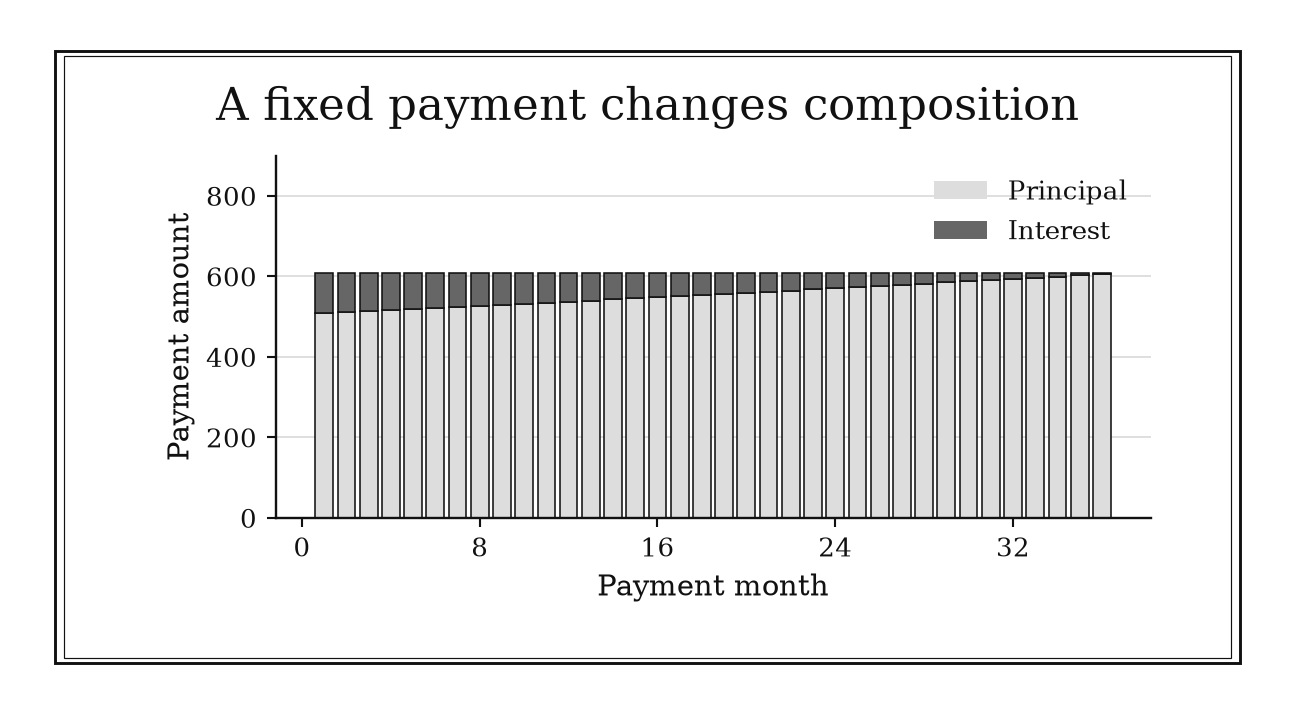
Figure 17.3. For a 20,000 loan at 0.5 percent monthly over 36 months, each payment is about 608.44. Interest declines as the balance falls, while the principal share grows; fees are excluded.
17.3.6: Annuity-due values shift payments one period earlier
History
At a positive discount rate, assume a payment due at the start of a period arrives at the end instead, and the valuation comes out too low, a timing error easy to make and miss. Johan de Witt’s 1671 report to the States of Holland could not afford that slip: he attached survival probabilities to specific payment dates and discounted each amount by exactly when it was due. De Witt discounted each date as it fell; packaging that sensitivity into one identity, that shifting every payment one period earlier multiplies a stream’s value by (1+r), is later actuarial shorthand.
The equation
For the same number and amount of payments at a common rate, compare present values at time zero and future values at time (n):
The ordinary stream pays at periods (1,,n); the due stream pays at (0,,n-1).
How to read it
(PV_{due}) and (FV_{due}) describe a stream paid at the start of each period; (PV_{ordinary}) and (FV_{ordinary}) describe the same stream paid at each period’s end. Shifting every payment one period earlier means each is discounted one fewer time, or compounds one extra period, and both produce the multiplier (1+r). It is a timing shift, not an additional payment. The multiplier only applies when payments and amount are unchanged between the streams; it does not adjust for a contract that adds an extra deposit.
How to use it
An assisted-living facility manager is quoted a five-year lease requiring ($1{,}000) payments at the start of each year, against a competing ordinary-annuity lease valued at ($4{,}212.36) under a 6% rate, same payment and count. Using the unrounded ordinary-annuity factor, its value with payment in advance is
not the ordinary annuity’s ($4{,}212.36); using unrounded values, the start-of-year lease costs the equivalent of ($252.74) extra today. She flags that before signing, since forgetting the shift would understate the true cost. She verifies the lease holds to five level payments and nothing more; a separate deposit at signing would sit outside the (1+r) shift and need its own valuation. Because the shortcut applies to a particular payment convention inside annuity calculations, it is Specialized.
Chapter Synthesis
Financial arithmetic becomes reliable when every comparison shares a base. The Rule of 72 estimates a compounding scale, the Fisher relation separates money growth from purchasing-power growth, and loss recovery exposes percentage asymmetry. Each is fast because its model is narrow.
The deeper workflow is temporal normalization. Convert rates to compatible effective periods, draw dated cash flows, and move every amount to one valuation date. NPV then compares modeled benefits and costs with an opportunity-cost benchmark.
Geometric-series formulas compress recurring schedules. Ordinary annuities, perpetuities, growing perpetuities, savings accumulations, amortizing loans, and annuities due differ mainly in horizon, growth, and payment timing. The formula follows the timeline, not the other way around.
One-Page Toolkit
| Question | Rule | Critical condition |
|---|---|---|
| Rough doubling time? | (T_2/r_{%}) | Steady compounded rate, roughly 2%–15% |
| Purchasing-power return? | (r_{real}=(1+r_n)/(1+)-1) | Same period and relevant inflation basis |
| Gain after loss (L)? | (G=L/(1-L)) | Same capital base, no external flows |
| Annual effect of periodic rate? | (EAR=(1+i)^m-1) | Constant periodic rate and compounding |
| Present value of dated flows? | (PV=C_t/(1+r)^t) | Matching date, period, risk, and inflation conventions |
| Basic project screen? | Accept if modeled (NPV>0) | Credible forecasts and opportunity-cost rate |
| Level finite payments? | (PV=C[1-(1+r)^{-n}]/r) | End-of-period, level payments |
| Level infinite payments? | (PV=C/r) | First payment next period, (r>0) forever |
| Growing infinite payments? | (PV=C_1/(r-g)) | Stable growth and (-1<g<r) |
| Regular savings accumulation? | (FV=C[(1+r)^n-1]/r) | End-of-period deposits, constant rate |
| Fixed amortizing payment? | (C=Pr/[1-(1+r)^{-n}]) | Contractual periodic rate and payment count |
| Beginning-period version? | Multiply matching ordinary-annuity value by (1+r) | Exact one-period shift, same payments |
Decision Path
- Write the objective: quick scale estimate, valuation, affordability, or contract comparison.
- Draw a timeline and mark every amount, sign, date, and currency.
- Put rates on a common effective-period basis and decide whether amounts and rates are nominal or real.
- Move every cash flow to one valuation date. Use a geometric closed form only after recognizing an exact pattern.
- Check domain conditions: payment timing, (r>0), (r>g), fixed count, and compatible periods.
- Stress-test cash flows and rates. Add taxes, fees, default, liquidity, and constraints when relevant.
- Treat the number as a model output, not personal financial advice; escalate high-stakes decisions to contract-specific analysis and qualified professionals.
Transfer Problems
1. Inflation and a drawdown
An account loses 30%, then gains 25%, while the relevant price index rises 4% over the full interval. Starting from ($10{,}000), compute the ending nominal value, nominal total return, and exact real return. What gain from the post-loss balance would have been required merely to recover the starting nominal amount?
2. Two payment offers
Choose between ($12{,}000) today and twelve ($1{,}050) month-end payments. At an effective monthly opportunity-cost rate of 0.6%, compute the installment stream’s present value. Then identify at least three nonmathematical contract features that could reverse a purely NPV-based choice.
3. Savings timing and a loan
A borrower deposits ($300) at the beginning of every month for (36) months into an account modeled at 0.4% monthly, while paying a separate (36)-month, ($9{,}000) loan at 7.2% nominal compounded monthly. Calculate the savings future value and loan payment, explain both timing conventions, and state why the modeled account return should not be netted mechanically against the contractual loan rate.
Where These Ideas Reappear
Compound factors are the exponential growth laws of algebra and differential equations. Present value is a weighted sum, while annuity formulas are finite or infinite geometric series from analysis. Real-versus-nominal conversion is another example of replacing additive intuition with multiplicative ratios.
Discounted cash flow reappears in bond duration, actuarial survival models, project optimization, energy-system planning, and cost-effectiveness analysis. Sensitivity to (r-g) anticipates condition numbers: a small denominator makes an answer fragile. Scenario analysis and Monte Carlo methods connect uncertain financial cash flows back to probability and measurement uncertainty.
Historical Notes and Sources
The doubling shortcut is supported by the digitized catalogue record for Pacioli’s 1494 Summa de arithmetica. Fisher’s exact nominal-real relation and present-value framework are documented in the full text of The Theory of Interest. The 1929–1932 drawdown context comes from Federal Reserve History.
Effective annual disclosure is documented in the Federal Reserve’s Regulation DD background and APY formula appendix. De Witt’s 1671 annuity work is reconstructed by the MacTutor history project and a peer-reviewed history of early annuity valuation.
The perpetuity example is grounded in the Bank of England archive’s consols ledgers; constant growth in Gordon and Shapiro’s 1956 paper; and mortgage institutional history in HUD’s official FHA history. No verified historical event is claimed for 17.3.4; that gap is recorded explicitly in the matching local story file.