Chapter 18: Applied Mathematics: Scaling, Regimes, and Model Sanity
If one term in an equation has units of energy and another has units of power, no amount of precise computation can make their sum physically meaningful. The model has failed before the solver starts. Applied mathematics often earns its greatest return by detecting that kind of failure early.
The same discipline extends beyond units. A credible model should recover known limiting cases, use variables scaled to reveal rather than conceal its structure, and retain the mechanisms that actually compete in the regime of interest. Dimensionless ratios turn those comparisons into portable numbers.
The fourteen rules in this chapter form a triage system. The first group tests equations and sensitivities before solving. The second reduces a model to characteristic scales, dimensionless groups, dominant balances, and timescale relationships. The third uses seven classic ratios to decide which physical picture deserves attention.
These ratios do not replace governing equations or experimental evidence. They select approximations and expose implausible ones. The governing habit is: check units and limits, choose honest scales, and identify the controlling regime before investing in a detailed solution.
18.1: Test the Model Before Solving It
Solving the wrong equation more accurately only deepens the error. These three rules screen structural consistency, known limits, and parameter sensitivity before algebra, fitting, or simulation creates false confidence.
18.1.1: Reject equations that are not dimensionally homogeneous
History
A single interface number carried the wrong unit: pound-force seconds where the code expected newton seconds. On 23 September 1999, Mars Climate Orbiter approached the planet on a trajectory far lower than planned, and NASA lost contact entering Mars. The mishap board traced the loss to that interface: ground software computed thruster impulse in the imperial unit, the navigation system read it as the metric one, and checks failed to catch it before encounter. Checking dimensions at every interface where a physical model connects subsystems is the discipline this rule generalizes.
The equation
A valid addition requires matching dimensions:
Arguments of logarithms, exponentials, and trigonometric functions must be dimensionless; for example,
Here ([Q]) denotes the dimension of (Q), not its numerical unit label.
How to read it
A physical law cannot change simply because meters are swapped for feet, so every term added or equated must carry the same dimensions: the same kind of quantity, such as length or force, regardless of the numeral attached. The same holds inside a logarithm or exponential: that argument must be a pure number. The check catches a wrong term instantly, the way a recipe calling for both cups and grams of flour would look off. It does not catch everything: an equation can pass and still describe the wrong physics. Passing it is necessary, never sufficient alone.
How to use it
A construction engineer commissioning a tower-crane hoist receives the vendor’s position formula: (x=x_0+vt+12at). Checking dimensions: (vt) works out to (()()=), but (at) works out to ((^2)()=), so it fails before a single test lift. Multiplying by another (t) turns (at) into (12at2=(2)(^2)=), restoring homogeneity, so she rejects the file. Passing confirms the terms can legally be added; it does not confirm the acceleration value is right, so she checks that constant against the motor’s spec sheet. This rule is an essential model-validation step rather than a complete physical test. Workflow.
18.1.2: Test every model in easy limiting cases
History
A theory bold enough to replace Newton’s gravity would be worthless if it could not still explain a dropped apple. Albert Einstein’s 1916 foundation paper on general relativity required the new field equations to recover ordinary Newtonian gravity in the weak-field, slow-motion limit, the regime where the older theory had succeeded. Passing that check did not prove relativity correct; it showed only that it did not contradict what was known. Testing a model in its easy limits before trusting untested predictions generalizes that requirement.
The equation
Choose a parameter limit that removes or dominates one mechanism and compare with a simpler result:
A model may also need to satisfy exact symmetries or conservation statements at special values.
How to read it
Send a model to a limit where the answer is already known, a parameter at zero or two quantities forced equal, the way a dimmer turned all the way down should leave a light off. These cases silence some terms, leaving a result checkable by hand. If the model fails, something is broken: a wrong sign, a missing factor, a coding slip. It cannot certify behavior away from that point; some limits are singular, meaning a small quantity set to zero can change how many boundary conditions the problem needs.
How to use it
A biomedical engineer is validating vendor software for a hypothermia-therapy cooling blanket before it reaches an ICU. The heat-loss term is (Q=hAT), with (h) the convection coefficient and (A=1.8) m(^2) skin area. Setting (h=0) should give (Q=0(1.8)T=0) for any (T); the vendor’s code instead returns (Q=12) W, a leftover baseline term never removed, enough to reject the release. The equal-temperature case, skin equal to ambient, passes cleanly. Passing confirms correct behavior at that extreme; it leaves open whether (h) was measured correctly, so she still validates it against a bench calibration. This rule is a reusable validation step that can disqualify a model but cannot prove it uniquely correct. Workflow.
18.1.3: Report parameter sensitivity as a dimensionless elasticity
History
Compare a one-dollar change in the price of salt with a one-dollar change in the price of a car: same units, wildly different businesses. Alfred Marshall’s 1890 Principles of Economics solved that mismatch, describing demand as more or less elastic by how strongly quantity bought responded to price, a ratio of percentage changes rather than raw amounts. Treating any output’s percentage response to any input’s change the same way is a modern extension of his comparison, not Marshall’s own claim.
The equation
For nonzero output (Q) and parameter (p), the local elasticity is
For a small relative change,
How to read it
Elasticity is the percent change in an output for each one percent change in an input, like grading a raise by percentage so a clerk’s raise and an executive’s sit on the same scale. It takes the plain rate of change and rescales it by (p/Q) so units cancel. An elasticity of (-1) means a one percent rise in input predicts about a one percent fall in output, near that point only. It is a local slope, not a curve, and can shift as the input moves far from where measured.
How to use it
A maple-syrup producer bottling by hand tracks flow through the fill spout, laminar pipe flow with (Q^{-1}), so flow’s elasticity with respect to viscosity is exactly (-1). A cooler overnight temperature raises viscosity (3%); (Q/QE_{Q,}(/)=(-1)(0.03)=-0.03) predicts a (3%) fall, and the actual (2.9%) drop is consistent with that viscosity effect if pressure and spout geometry stayed fixed. She checks those conditions before warming the syrup; agreement alone cannot rule out clogging. A swing large enough to leave the laminar regime would make (-1) stop describing the real response. This rule directly produces a portable local sensitivity measure. Independent.
18.2: Strip a Model Down to Its Governing Scales
Scaling turns a page of dimensional terms into a small set of comparisons. It reveals which effects compete, which variables are poorly normalized, and where different approximations must meet.
18.2.1: Scale variables so typical dimensionless values are order one
History
Stretching the coordinate near a solid wall the right way turns a flow equation that looks hopeless into two solvable pieces. At the 1904 International Congress of Mathematicians, Ludwig Prandtl argued that flow with very small viscosity still develops a shrinking zone hugging the surface, where viscous effects cannot be ignored. His move stretched the near-wall coordinate until the invisible viscous term became ordinary size again inside that zone. Picking scales that keep variables neither vanishing nor exploding generalizes that rescaling.
The equation
Choose characteristic scales (L,T,U) and write
so typical dimensionless variables satisfy
How to read it
Pick a typical size for each quantity, a length (L), a time (T), a speed (U), then measure everything as a multiple of that size instead of raw meters or seconds, a step called nondimensionalizing, the way a recipe scaled to servings reads better than one scaled to grams. In the regime you care about, the result should sit near (1), neither huge nor tiny. “Order one” means that comfortable middle size, not exactly (1.0). This step alone does not solve anything: it rearranges the equation so coefficients compare honestly. A single global scale can also hide a thin region needing its own smaller characteristic size to become visible.
How to use it
An instrumentation specialist is setting up a simulation for a pressure-sensor diaphragm (2) mm across, using a geometry file inherited from a template built in meters. The diaphragm’s coordinates sit near (2^{-3}), so absolute geometry tolerances inherited from a meter-scale model need checking; that magnitude alone does not exhaust floating-point precision. She rescales, choosing (L=2^{-3}) m, so (x=x/L) runs from (0) to (1) instead of (0) to (0.002). She transforms coefficients and tolerances consistently and converts outputs back to physical units. The scaling makes numerical scales easier to compare; convergence checks must establish whether stress and strain accuracy improved. A later variant a tenth as thick would need its own characteristic length. Because scaling prepares later asymptotic and numerical work, it is a Workflow rule.
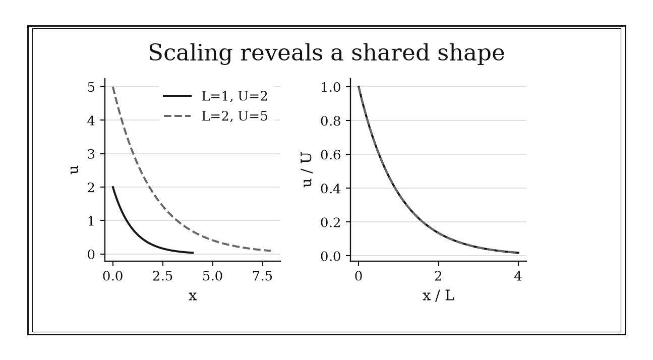
Figure 18.1. Two constructed profiles u(x)=U exp(-x/L), with different U and L, collapse to the same curve when plotted as u/U against x/L. Collapse follows from their shared model, not from scaling arbitrary data.
18.2.2: Reduce dimensional variables with Buckingham Pi
History
Two engineers running the same scale test could defend opposite conclusions, with no rule for whose numbers transferred between models and full-scale systems. In 1914, working in Washington, D.C., Edgar Buckingham published “On Physically Similar Systems,” showing any relation among several dimensional quantities can be rewritten using a smaller set of dimensionless combinations. Two systems sharing those numbers behave alike regardless of size; textbooks after him named the result the Buckingham Pi theorem.
The equation
If a relation involves (k) dimensional variables whose dimension-exponent matrix has rank (r), then
Each group has the form (_j=i q_i^{a{ij}}) with exponents in the null space of the dimension matrix.
How to read it
Every independent physical dimension in a list of quantities, such as mass, length, and time, imposes one constraint on how their exponents can combine. Solving those constraints leaves a set of products, like speed times length divided by viscosity, whose units cancel completely: a pure number. The theorem specifies how many such products a list must yield; it does not reveal the relationship between them. Leaving an important variable out is invisible to the theorem: it reduces whatever list you hand it, right or incomplete.
How to use it
A cycling team’s aerodynamics analyst measures drag on a rider in a wind tunnel and wants to know how many independent numbers describe the result. Drag depends on force (F), density (), speed (U), body length (L), and viscosity (), so (k=5) quantities spanning three base dimensions, rank (r=3), predicting (k-r=5-3=2) groups. She builds drag coefficient (C_D=F/(U2L2)) and Reynolds number (Re=UL/); one curve of (C_D) against (Re) predicts drag at any speed sharing that Reynolds number. Leaving out a relevant variable would still yield the same count, quietly hiding a real effect inside apparent scatter. This rule directly compresses any dimensionally homogeneous variable list. Independent.
18.2.3: Find leading behavior by balancing the largest competing terms
History
Drop viscosity from a flow equation because it is small almost everywhere, and you can lose the region that decides the answer. Ludwig Prandtl faced that puzzle at the International Congress of Mathematicians on 12 August 1904 in Heidelberg, Germany: viscosity is negligible across most of a fast-moving flow, yet a thin layer next to a solid surface behaves differently, because steep velocity changes there make viscous forces comparable to inertia. Weighing those two terms directly against each other let Prandtl keep the necessary no-slip behavior instead of erasing it.
The equation
For candidate terms (A,B,C), posit
for every term (C) to be neglected. The inferred scales must make the assumed ordering self-consistent.
How to read it
A model often reduces to comparing two terms that must be roughly equal in size, the way a seesaw balances only when both sides push back equally. Setting those terms equal, symbol for symbol, lets you solve for a scale you did not know in advance, such as how thick a transition layer must be. That guessed scale is not automatically right: substitute it back into every other term and confirm each is small. A term that looks large from its raw coefficients can still vanish through cancellation, so size alone is not proof it matters.
How to use it
A civil engineer studying a simplified transport layer near a bridge pier first uses the illustrative equation (y’‘+y’=0), where () comes from flow speed, water viscosity, and pier width. Balancing the retained terms, (/^21/), gives thickness (); times length (L=0.5) m gives (0.0016=0.0008) m, under a millimeter, as the layer scale in this toy model. Discarding the second-derivative term everywhere would erase the layer; predicting sediment deposition or scour also requires the boundary conditions, wall shear, and an appropriate sediment-transport model. This rule directly estimates governing scales across models. Independent.
18.2.4: Compare process timescales before coupling models
History
A boundary layer is as much a clock as a place: inside it, momentum adjusts almost immediately; further out, the same adjustment can take far longer. Prandtl’s 1904 paper stops at the split itself: a fast-responding region at the surface, a slower outer flow. Clocking the two regions separately, so a fast piece can be swapped for a simple algebraic stand-in once it settles, is this rule’s extension.
The equation
Let (T_f) and (T_s) be characteristic fast and slow times:
A fast-slow model may be written
suggesting (g(x,z)) after a stable fast transient.
How to read it
Compare two characteristic times: how long the fast process takes to settle, (T_f), against how long the slow process takes to noticeably change, (T_s). Their ratio, (=T_f/T_s), is small when the fast process is quicker by a factor of ten or more. If stable, the fast process appears on the slow clock to snap almost instantly to wherever the slow variables sit, letting you replace it with a simpler algebraic relation. Smallness alone is not enough: an unstable fast process can refuse to settle, and comparing against total experiment length can make it look artificially slow.
How to use it
A grid battery’s current settles far faster than its temperature does; the control engineer needs to know if that gap allows separate models. Current settles in about (T_f=1) ms, temperature in about (T_s=10) s, giving (=T_f/T_s=10{-3}/10=10{-4}). Because the response is also stable, the engineer treats the electrical state as quasi-steady inside the thermal model. The shortcut assumes no fast-repeating cycling; a drivetrain pulsing every few milliseconds would re-excite the transient before it settles, forcing the full coupled model. This is a model-reduction workflow step. Workflow.
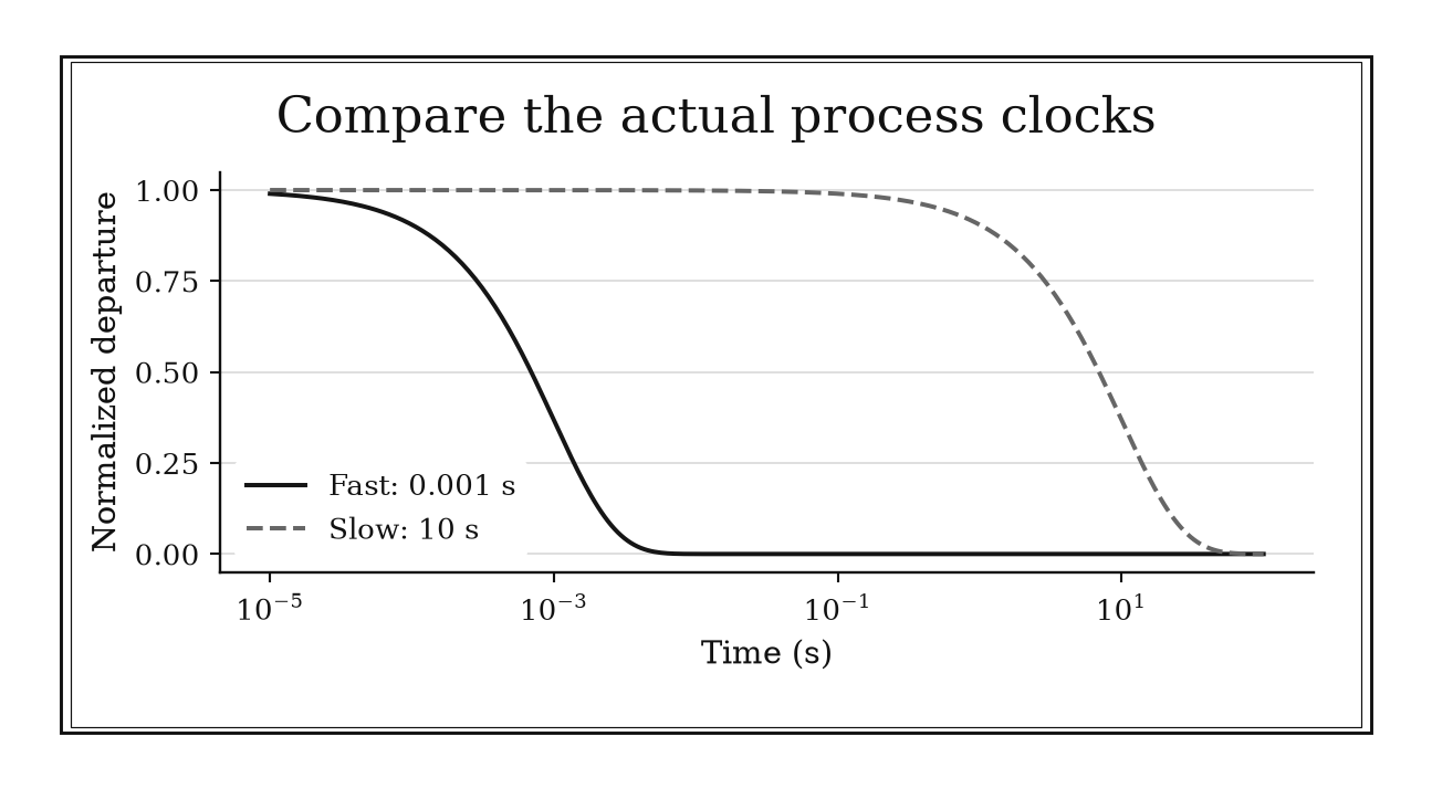
Figure 18.2. Stable constructed decays with time constants 0.001 s and 10 s settle on very different clocks. A fast state can be treated as relaxed only after its transient, and renewed forcing can excite it again.
18.3: Use Ratios to Select the Right Physical Regime
Dimensionless numbers compare mechanisms on the chosen scales. They are regime selectors: each says what may dominate, what might be neglected, and which approximation deserves a closer test.
18.3.1: Use Reynolds number to compare inertia with viscosity
History
Sizing a pump for smooth pipe flow can leave it struggling against a turbulent regime that costs far more energy to move the same water. In 1883, working in Manchester, Osborne Reynolds injected a visible dye filament into water flowing through a glass pipe and varied its speed and diameter. At low speed the dye ran straight; as speed rose, it broke into a tangled smear. This transition occurred near the same value of a dimensionless combination of speed, size, density, and viscosity, though Reynolds did not claim one universal number for every geometry.
The equation
where () is density, (U) characteristic speed, (L) characteristic length, () dynamic viscosity, and (=/) kinematic viscosity.
How to read it
Rewriting the equation of motion for a fluid in ratios instead of raw units, nondimensionalizing, turns speed, size, density, and viscosity into one number, the Reynolds number, comparing the fluid’s own momentum against internal friction. A small value favors thick, orderly motion; a large value permits shear layers and eventually turbulence, though large alone guarantees none specifically. Length (L) must match the geometry, a pipe’s diameter for round pipes, hydraulic diameter for an odd duct. This number sorts flows into rough families; it does not hand you the exact transition speed.
How to use it
A municipal water utility operator is sizing a new water main, unsure whether the flow will behave like the smooth motion of a slow leak or the churned mixing governing pump losses. At the design flow, water moves at (U=1) m/s through a pipe of diameter (L=0.10) m, kinematic viscosity (^{-6}) m(^2)/s. The Reynolds number is (Re=UL/(0.10)/10{-6}=105), far above any documented transition, so she rules out a laminar model and pulls correlations built for turbulent flow. The number alone does not say how rough the pipe’s interior is; she still looks up a roughness correlation first. Because it guides model selection rather than finishing the analysis, this is a Workflow rule.
18.3.2: Use Peclet number to compare advection with diffusion
History
Molecular diffusion alone badly underestimates how far a dissolved substance travels through a moving fluid. G. I. Taylor’s 1953 analysis, based in Cambridge, United Kingdom, examined solute carried through a tube by flowing water: sideways diffusion moved material between the tube’s faster center and slower edges, while flow carried it downstream. Taylor compared those two effects directly; naming their ratio a Péclet number is this book’s packaging, not his term. Their combined interaction produced spreading far larger than diffusion alone could explain.
The equation
where (T_{adv}=L/U) and (T_{diff}=L^2/D). For heat transfer, thermal diffusivity () replaces (D).
How to read it
Compare two competing times over the same distance: how long molecular diffusion takes to spread material across a length (L), against how long the bulk flow takes to carry it past that length. Their ratio is the Péclet number, the way a drop of ink either spreads evenly or gets swept downstream in a current before it can. Much greater than one, as usual beyond microscopic scales, the flow outruns that diffusion mechanism; whether sharp fronts persist also depends on shear, dispersion, and other mixing. The number depends on direction and length: it can be enormous along the flow while modest across a channel, so one value can hide which direction controls the mixing.
How to use it
An environmental engineer is estimating whether molecular diffusion alone can homogenize a contaminant plume moving through a one-meter monitoring interval in a shallow aquifer. Groundwater moves at (U=10^{-5}) m/s, interval length (L=1) m, diffusivity (D=10^{-9}) m(^2)/s. The Péclet number is (Pe=UL/D=10{-5}(1)/10{-9}=10^4). With (Pe) that large, diffusion cannot smooth the plume across that meter during transit, so molecular diffusion alone cannot justify a well-mixed model. She also checks mechanical dispersion and heterogeneity before setting well spacing or treating the front as sharp. The Péclet number describes transport along the flow only; a smaller cross-channel scale could give genuine local mixing it does not capture. This ratio is a regime-selection workflow step. Workflow.
18.3.3: Use Damkohler number to compare reaction with transport
History
A nearly uniform reactor can turn into one where almost all conversion happens near the inlet, the moment a reaction’s own speed outpaces how fast material moves through the vessel. In November 1940, Gerhard Damköhler analyzed turbulent flame speed by comparing turbulent mixing against the chemical burning reaction, organizing combustion behavior by which process could act first. Later research kept this comparison as a way to classify reacting flows, though several Damköhler numbers are in use depending on which mechanism is compared.
The equation
In general,
For a first-order reaction with rate constant (k) and advective residence time (L/U),
Diffusion-controlled problems use a different transport time and therefore a different expression.
How to read it
Material takes some time to move through or mix in a system; the reaction has its own characteristic timescale. Their ratio is the Damköhler number. A large value means reaction is fast relative to the chosen transport mechanism; whether that leads to depletion or approach to a reversible equilibrium depends on the kinetics. A small value means material moves through, or mixes away, before much reaction happens. Whether a value counts as large or small depends entirely on which kinetics and transport mechanism built the two times; the same system can report a different number under an equally valid definition.
How to use it
A process engineer at a chemicals plant is deciding whether a plug-flow reactor can be modeled as reaching near-complete conversion, or needs a fuller kinetic model. The reaction has rate constant (k=2) s(^{-1}), residence time (T_{res}=0.10) s. The Damköhler number is (Da=kT_{res}=2(0.10)=0.20). For ideal first-order conversion, the fraction converted is (1-e{-Da}=1-e{-0.20}=0.181), about (18%) per pass. Assuming near-complete conversion would badly overstate output, so she sizes downstream separation equipment around this modest conversion instead. The (0.20) figure describes only this kinetics and residence-time definition; a different reaction order would need its own recomputed number. This is a regime-selection Workflow rule.
18.3.4: Use Fourier number to estimate diffusion penetration time
History
How far heat has actually traveled into a roast, a cast wall, or a quenched metal part after a given time is a question intuition and calculation can answer very differently, and before 1822 there was no agreed way to settle it. Joseph Fourier’s Théorie analytique de la chaleur, published that year in Paris, related temperature’s evolution to geometry, material, and elapsed time: penetration distance grows with the square root of diffusivity times time, not time itself. Later engineers named that ratio the Fourier number; Fourier’s own treatise used none of that terminology. His result still turned a guess into a calculable quantity.
The equation
where () is thermal or mass diffusivity, (t) elapsed time, (L) system scale, and (_d) a penetration scale.
How to read it
Balancing how fast temperature changes against how fast that change diffuses shows a disturbance’s reach into a body, (_d), grows like the square root of diffusivity () times elapsed time (t), not in direct proportion to time. The Fourier number packages that as (t/L^2), comparing elapsed time against the time diffusion needs to cross (L). Near one means diffusion has had roughly enough time to reach across that length, not that temperature is perfectly even; corners still leave real unevenness. Whether (L) means full thickness, half-thickness, or a radius changes the numbers by a large factor.
How to use it
A canning supervisor has one batch to confirm how long a jar of dense preserve must sit in a hot-water bath before heat has penetrated to its center, given half-thickness (L=0.01) m and diffusivity (^{-7}) m(^2)/s. The diffusion time is (L2/=(10{-2})2/1.4{-7}) s, about twelve minutes. After just (1) s, penetration is only (_d=) mm, so she extends the hold time. The Fourier number tells her when heat has had time to reach the center; it does not guarantee that center reached food-safe temperature, which depends on boundary temperature and geometry, not time alone. This rule directly estimates a portable diffusion scale. Independent.
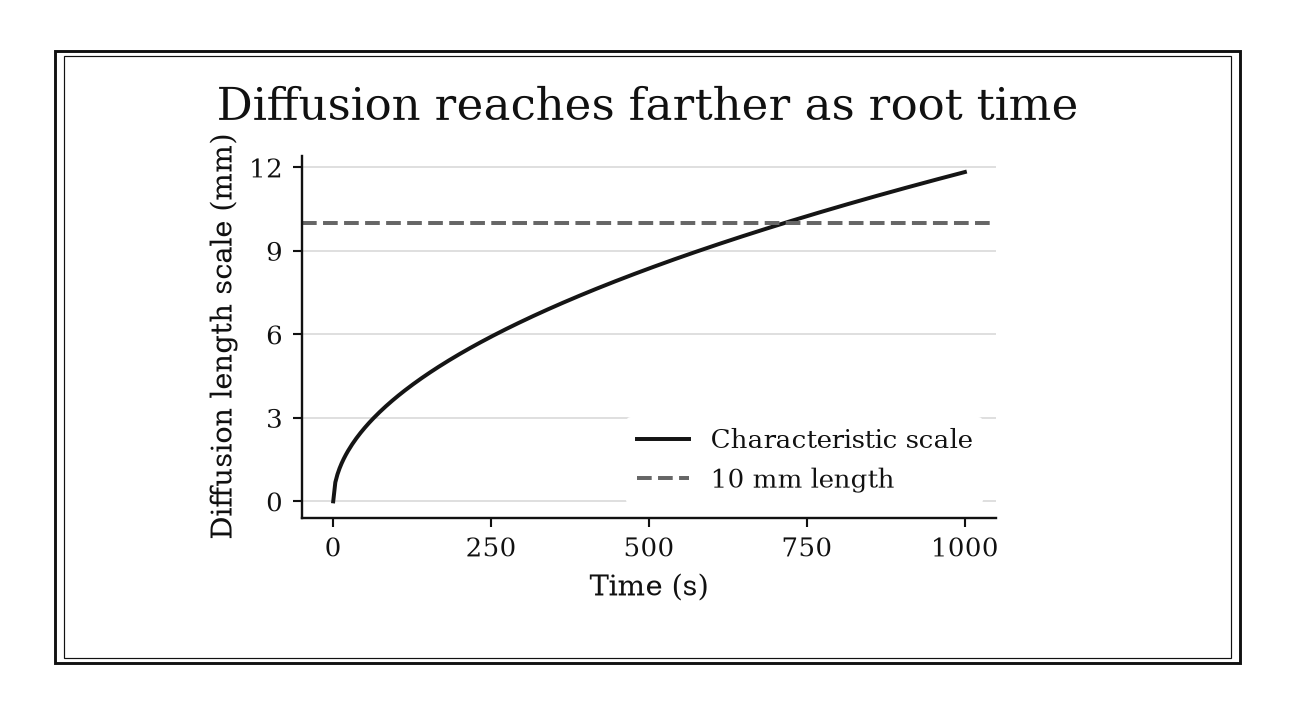
Figure 18.3. The characteristic length sqrt(alpha*t), with alpha=1.4×10^-7 m²/s, reaches 10 mm near 714 s. This scale is not a temperature threshold or a safety certificate.
18.3.5: Use lumped thermal capacitance only for small Biot number
History
Some heated or quenched parts can be trusted to hold one uniform temperature throughout; others cannot, and only hard series solutions, worked one geometry at a time, could tell which. M. P. Heisler’s 1947 paper, published in New York, gave engineers practical charts for transient temperatures in plates, cylinders, and spheres, organized by dimensionless time and the ratio of internal to surface resistance, without declaring the modern one-tenth cutoff a universal law. The modern Biot-number screening rule interprets that distinction as a quick test.
The equation
where (h) is convection coefficient, (k_s) solid conductivity, and (L_c) the volume-to-surface characteristic length.
How to read it
The Biot number compares two resistances to heat flow: how hard it is for heat to move through a solid’s interior by conduction, against how hard it is to cross into the fluid by convection. When conduction resistance is much smaller, heat spreads through the interior quickly enough that treating the whole solid as one temperature, updated over time, is a reasonable shortcut. The common one-tenth cutoff reflects tolerable unevenness, not a fixed law. A small Biot number says the body is nearly uniform at a moment; it leaves the process duration open, since that depends on thermal mass too.
How to use it
A batch of copper fittings is headed into the quench bath; the foreman needs to know if one quench temperature fits all, or if a full internal simulation is required. The bath gives (h=2000) W/m(^2)K, a liquid quench, length (L_c=V/A_s=0.01) m, conductivity (k_s=400) W/mK. The Biot number is (Bi=hL_c/k_s=2000(0.01)/400=0.05), still below the one-tenth threshold, so he commits to the lumped model: every fitting tracked with one temperature. The lumped model does not confirm the surface actually sees the assumed (h); a fitting touching neighbors in a rack would need rechecking. This ratio is a model-selection Workflow rule.
18.3.6: Check Mach number before neglecting compressibility
History
A spark-lit photograph showed what a fast-moving projectile does to the air around it: disturbances trailing behind, invisible but plainly there on film. On 21 April 1887 in Fiume, then Austria-Hungary and now Rijeka, Croatia, Ernst Mach and Peter Salcher used spark photography to capture these disturbances; later engineers drew today’s incompressible-flow cutoff, a line the pair themselves never marked. Their photographs still helped establish speed relative to sound as the scale controlling the divide between subsonic and supersonic motion.
The equation
where (U) is characteristic flow speed and (a) is the local speed of sound. For an ideal gas, (a=), where () is the heat-capacity ratio, (R_s) is the specific gas constant, and (T) is absolute temperature.
How to read it
Mach number compares how fast something moves through a gas with how fast pressure disturbances travel through it, the speed of sound. As that ratio climbs, the gas increasingly cannot get out of the way instantly: density changes noticeably, and past a point shocks, abrupt jumps in pressure and density, appear. The often-quoted cutoff near Mach (0.3) for constant density is a convenience tied to tolerable density change, not a hard boundary. A low bulk Mach number does not guarantee constant density everywhere: local heating can produce real variation while the flow moves slowly.
How to use it
A fixed-wing delivery drone nearing cruise design freeze needs simpler incompressible formulas or full compressible modeling; the logistics company’s engineers must decide which applies. At the planned cruise speed (U=50) m/s, speed of sound (a=340) m/s, the Mach number is (Ma=U/a=50/340=0.147), comfortably inside the incompressible range, so the team proceeds with simpler design tools. That bulk figure is the cruise speed; local speeds over a curved wing run faster, so a part safely subsonic in bulk can still see locally compressible flow. This ratio is a model-selection Workflow rule.
18.3.7: Check Knudsen number before using continuum equations
History
A vacuum system or narrow channel designed on ordinary fluid-flow assumptions can deliver a flow rate wrong by a large factor as pressure drops. In 1909, working in Copenhagen, Martin Knudsen measured gas flow through tubes and traced the breakdown of standard viscous-flow predictions to a single comparison: how far a gas molecule travels, on average, before colliding with another, against the tube’s size. That transition, established directly by Knudsen, moved flow toward molecules bouncing individually off the walls; today’s numerical boundaries are later conventions.
The equation
where () is molecular mean free path and (L) is the smallest relevant geometric or gradient length.
How to read it
Ordinary continuum equations for fluid flow assume a gas molecule collides with many other molecules over the distance across which pressure, velocity, or temperature meaningfully changes. The Knudsen number, the ratio of a molecule’s average travel distance between collisions to that geometric distance, measures how good that assumption is. When tiny, molecule-molecule collisions vastly outnumber collisions with a wall, and the no-slip picture holds well. As it grows, molecule-wall collisions matter as much, and assumptions like zero gas velocity at a surface fail before the bulk conservation laws stop being useful. Mean free path changes with pressure, so one device can read small in one region and much larger in a throat.
How to use it
A new etch tool’s gas-delivery microchannels need sizing, and the semiconductor-equipment manufacturer must know whether standard continuum equations apply or rarefied-gas effects dominate. The process gas has mean free path () nm; the channel is (10) micrometers wide, so (L=10^{-6}) m. The Knudsen number is (Kn=/L=70{-9}/(10{-6})=0.007), near the edge of the continuum range, so engineers keep the design but flag it for a slip-flow correction. Mean free path shifts with local pressure, so a channel safely continuum near its inlet can still develop a much larger Knudsen number at a throat downstream, unseen by the inlet calculation. This ratio is a model-selection Workflow rule.
Chapter Synthesis
Applied mathematics starts with rejection tests. Dimensional homogeneity catches incompatible terms and interfaces. Limiting cases demand correspondence with simpler truths. Elasticity turns local parameter response into a unit-free comparison.
Scaling then exposes structure. Order-one variables remove arbitrary magnitudes, Buckingham Pi reduces variable count, dominant balance finds governing terms, and timescale ratios identify fast and slow subsystems. Each reduction must be substituted back into the full model and tested for self-consistency.
Finally, dimensionless ratios select physical regimes. Reynolds, Péclet, Damköhler, Fourier, Biot, Mach, and Knudsen numbers compare mechanisms, not merely labels. Their values matter only with clearly defined scales, geometry, properties, and accuracy goals.
One-Page Toolkit
| Question | Ratio or rule | What it screens |
|---|---|---|
| Can these terms coexist? | Require matching dimensions | Structural consistency, not physical truth |
| Does the model recover known behavior? | Test zero, equal, small, and large limits | Signs, factors, missing mechanisms, code defects |
| How sensitive is output proportionally? | (E_{Q,p}=(p/Q)Q/p) | Local percent response |
| Are numerical magnitudes revealing structure? | Scale typical variables to (O(1)) | Conditioning and coefficient comparisons |
| How many independent groups remain? | (k-r) Buckingham groups | Dimensional reduction |
| Which terms set a scale? | Balance comparable leaders; verify all neglected terms | Asymptotic regime |
| Can a fast subsystem be reduced? | (T_f/T_s) plus stable fast dynamics | Quasi-steady approximation |
| Inertia or viscosity? | (Re=UL/) | Flow regime |
| Advection or diffusion? | (Pe=UL/D) | Transport layers and mixing |
| Reaction or transport? | (Da=T_{transport}/T_{reaction}) | Conversion regime |
| How far has diffusion penetrated? | (Fo=t/L^2), (_d) | Transient scale |
| Is a body nearly uniform in temperature? | (Bi=hL_c/k_s) | Lumped thermal model |
| Is compressibility negligible? | (Ma=U/a) | Density and wave effects |
| Is continuum/no-slip physics credible? | (Kn=/L) | Rarefaction and kinetic effects |
Decision Path
- Define the output, domain, and decision accuracy. List variables with units.
- Check dimensional homogeneity, signs, conservation, symmetries, and easy limits before solving.
- Choose characteristic scales that make typical variables order one; allow different scales in different regions.
- Form independent dimensionless groups and identify plausible dominant balances.
- Compute relevant regime ratios with explicitly defined (U,L,T), properties, and geometry.
- Select the simplest model consistent with those ratios, then substitute the approximation back into every discarded term.
- Compare with data or a higher-fidelity model near thresholds; escalate when multiple ratios are order one or uncertainty crosses regimes.
Transfer Problems
1. A proposed cooling law
A model claims (T(t)=T_+(T_0-T_)e^{-ht}), where (h) is stated in W/m(^2)K. Diagnose the dimensional problem, construct the lumped-capacitance exponent using the missing physical quantities, and list the Biot and limiting-case checks required before using it.
2. Reaction in a microchannel
Water carries a dilute reactant through a (100) ()m-wide, (5) cm-long channel at (0.01) m/s. Given (D=10^{-9}) m(^2)/s and first-order (k=0.2) s(^{-1}), compute axial and transverse Péclet numbers and an advective Damköhler number. Explain why a single length choice cannot answer every transport question.
3. High-altitude small-scale flow
A (1) mm probe moves at (250) m/s where (a=300) m/s, (^{-5}) m(^2)/s, and () ()m. Compute (Ma), (Re), and (Kn). Identify which common continuum, incompressible, and viscous assumptions are threatened, and propose the next model checks rather than selecting a solver immediately.
Where These Ideas Reappear
Dimensional homogeneity and limiting cases are universal tests in physics, engineering, statistics, and software. Elasticity is logarithmic differentiation from calculus and connects directly to uncertainty propagation. Buckingham Pi is linear algebra on a dimension-exponent matrix, while dominant balance and multiple scales lead into asymptotic analysis and differential equations.
The seven regime numbers recur in heat transfer, fluid dynamics, chemical engineering, microfabrication, environmental transport, and numerical PDEs. Their shared pattern, effect A divided by effect B, also appears in signal-to-noise ratios, condition numbers, and optimization tolerances. Near a regime boundary, uncertainty in inputs becomes uncertainty in model class.
Historical Notes and Sources
The model-failure and correspondence stories are documented in NASA’s Mars Climate Orbiter Mishap Investigation Board report and Einstein’s 1916 foundation paper. Elasticity is supported by Marshall’s chapter on elasticity. Scaling and dominant balance draw on the NACA translation of Prandtl’s 1904 boundary-layer paper, while dimensional reduction follows Buckingham’s 1914 paper.
The transport-regime histories come from the primary records of Reynolds’s 1883 pipe experiments, Taylor’s 1953 dispersion analysis, and Damköhler’s 1940 flame paper. Diffusion scaling is grounded in the digitized 1822 Fourier treatise, and lumped-capacitance history in Heisler’s 1947 paper.
High-speed and rarefied-flow episodes are documented in a history of the Mach–Salcher experiment and Knudsen’s 1909 paper. These are the sources recorded in the matching local research and historical-story files; modern cutoff values and compact rule wording are presented as later interpretations.