Chapter 19: Optimization: Scale, Search, and Certify
A design variable measured in meters is replaced by the same quantity in millimeters, and an optimizer that had seemed calm begins taking erratic steps. The physical problem has not changed. Its numerical landscape has. Gradients, curvature, stopping tolerances, and regularization all inherit the coordinates in which the problem is written.
That observation separates optimization from merely pressing “solve.” A successful run begins by preparing the geometry, continues with a search that can recover when its local model is wrong, and ends with a certificate matched to the problem’s constraints and convexity. A flat progress display is not proof of optimality; it may signal poor scaling, stochastic noise, an unsafe step, or the wrong residual.
The nineteen rules in this chapter follow that sequence. The first five scale variables, features, stable expressions, curvature, and stochastic error. The next six choose and globalize local search methods. The final eight verify derivatives and demand a defensible reason to stop.
The governing habit is: prepare the coordinates, test each step against observed behavior, and certify the result with conditions the problem actually satisfies.
19.1: Prepare the Landscape
Optimization algorithms see coordinates, not physical meaning. Unit choices can distort curvature, exponentials can overflow before an objective is evaluated, and gradient noise can impose a floor no deterministic stopping test can cross. These rules make the landscape numerically legible before method tuning begins.
19.1.1: Nondimensionalize optimization variables before tuning
History
A solver that converges quickly in one set of units can crawl to a near halt after nothing but a change of units. Dong Liu and Jorge Nocedal met a version of this in August 1989, in Evanston, Illinois, while testing a large-scale optimization method storing only a short history of past steps instead of a full curvature matrix. They found a simple scaling choice accelerated convergence, a lesson that generalizes: units and magnitudes shape the geometry every optimizer sees.
The equation
Choose characteristic scales and write
Derivatives transform as
Bounds, constraints, priors, and penalties must be transformed with the variables.
How to read it
Here is the variable in its own natural unit: divide the raw value by a characteristic size so the result is a plain number near one, the way cups describe a recipe better than fluid ounces of a pool. With every rewritten variable near one, a single stopping tolerance means roughly the same thing in every direction.
The rule does not pick the right characteristic size for you: a scale far from the values the design will take can look near-one and still hide bad scaling, and any bound or penalty carried along must be rescaled too.
How to use it
Thickness near meters and elastic modulus near pascals, a measure of how strongly the material resists stretching, sit apart. A structural engineer sizing a composite panel for a pedestrian bridge hands both to a gradient-based optimizer, a routine that repeatedly nudges the design toward lower cost: one step size safe for one variable is reckless or paralyzed for the other. Choosing and rewriting both as puts them on the same footing.
Setting to the current guess, rather than the panel’s plausible range, can make a 1-millimeter design look well-scaled and then go poorly scaled once the search moves it toward 5 millimeters. This is a Workflow rule: nondimensionalization is a preparatory stage that makes later search and certification decisions comparable.
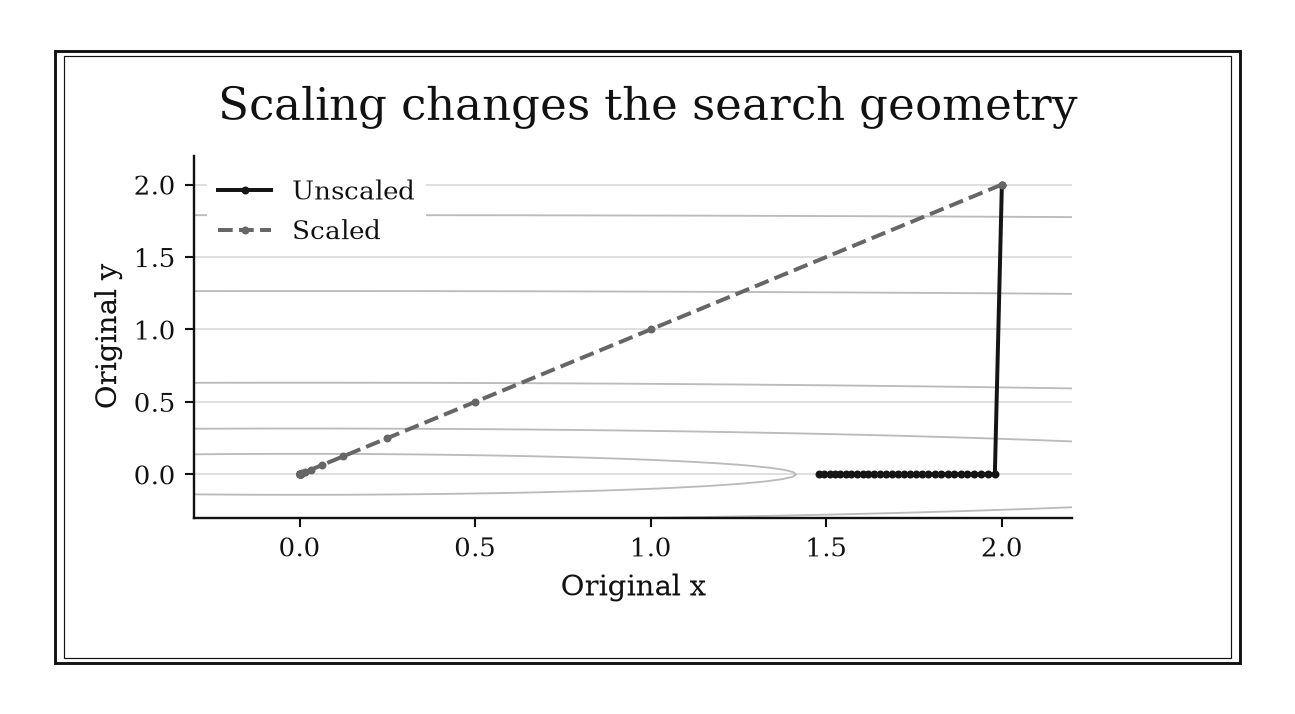
Figure 19.1. For f(x,y)=(x²+100y²)/2, gradient descent with step 0.01 sheds y error quickly but reduces x slowly. Scaling v=10y permits a balanced step; both paths are shown in original coordinates.
19.1.2: Scale features before coordinate descent
History
A column of lab-marker values a thousand times larger than a column
of patient ages is, to a coordinate-descent fitter, a louder voice in
the room, regardless of which predictor matters more for medical risk.
In January 2010, Jerome Friedman, Trevor Hastie, and Robert Tibshirani
published fast cyclic coordinate-descent algorithms, updating one
variable at a time in rotation, for regularized regression models. Their
glmnet software standardized predictors by default, keeping
penalized fits practical without feature units dominating the geometry.
Scaling predictors and adjusting penalties, done properly, are one
operation, not two.
The equation
For least squares
the coordinate curvature is
and a gradient-like coordinate update has the scale
For other smooth losses, use the appropriate coordinate Lipschitz bound.
How to read it
Each coordinate-descent update solves a small one-variable problem and moves that coefficient. A column with a large norm, meaning values spread over a wide range, produces a steep, narrow problem, so a raw step that barely moves one coefficient can send another wildly off course. Dividing the step by , a per-column curvature number, corrects for this.
The rule does not keep a penalty meaningful after rescaling: standardizing changes what a penalty costs a coefficient, so a penalty left at its old size while columns rescale underneath it stops meaning what it used to.
How to use it
A lab-marker column measured in milligrams per deciliter carries norm near 1000; an age column measured in years carries norm near 1. For a hospital data analyst fitting a regularized model to flag 30-day readmission risk, the resulting curvatures are and . An unscaled step is unstable for the marker and slow for age. The analyst standardizes both columns and rescales the lasso penalty to survive the transformation.
A sparse indicator, say a flag for prior surgery, has a small norm by construction, and standardizing it can inflate its importance past its real weight. The analyst leaves it unscaled and rescales inside each cross-validation fold, since scaling from the full data would leak information. This is a Workflow rule: feature scaling prepares coordinate descent and its penalty path rather than delivering a standalone scientific conclusion.
19.1.3: Shift by the maximum in log-sum-exp and softmax
History
Two formulas can be algebraically identical and still disagree the moment a computer evaluates them, one returning a usable number and the other silently overflowing. On 19 August 2020, Pierre Blanchard, Desmond Higham, and Nicholas Higham tested this pair of formulas for combining exponentials, the log-sum-exp and softmax expressions used throughout machine-learning models. Their experiments confirmed that shifting every input by its largest value blocks overflow, while uncovering subtler cancellation risks among other rewrites. The disagreement was never about the algebra; it was which arithmetic path survives finite-precision computation.
The equation
Let . Then
and the softmax probabilities are
The shift cancels from every ratio and is added back only to the logarithm.
How to read it
Log-sum-exp exponentiates each number in a list (raises to that power), adds the results, and takes the logarithm of the sum; softmax turns the list into probabilities adding to one. Both blow up once an input like 1000 is exponentiated directly, since exceeds what a computer can hold. Subtracting the largest input first keeps every value at zero or below, so nothing overflows, and adding back afterward restores the original answer.
This shift only fixes overflow. It says nothing about cancellation between nearly equal positive and negative exponential terms, a separate risk needing its own dedicated technique.
How to use it
A logistics dispatcher’s demand-allocation system scores two regional depots for an urgent shipment and must convert scores into a routing probability. The raw scores are 1000 and 999, and directly overflows before a probability can form. Subtracting the maximum, , gives , with the two probabilities and , so the shipment routes mostly through the first depot with a real share reserved for the second. The software applies this shift by default, since it costs nothing when scores are modest.
The shift does not rescue every case: combining positive and negative weighted exponentials can lose sign information distinguishing a favored depot from a disfavored one, and a specialized signed-arithmetic method is what handles that case. This is a Workflow rule: stable evaluation is a reusable component inside a larger objective, probability, or dynamic-programming calculation.
19.1.4: Condition number predicts gradient-descent speed
History
Why does one calibration crawl toward its answer for thousands of iterations while a similar problem snaps into place in dozens? In the early 1960s, Boris Polyak analyzed gradient methods, search procedures that repeatedly move a guess toward steeper cost reduction, and their acceleration. His analysis helped establish that curvature in the steepest and flattest directions sets how slowly such a method shrinks its error. The condition-number rate used today specializes that finding to smooth, bowl-shaped problems; it is not a universal speed law.
The equation
If is -smooth and -strongly convex with , define
Gradient descent with satisfies a bound of the form
How to read it
Picture the cost function as a bowl. measures how sharply it curves in its steepest direction and how gently in its flattest; a step safe for the steep direction is timid for the flat one. Their ratio, , the condition number, describes how stretched the bowl is: round means , a narrow valley puts in the thousands. Descent shrinks its error by a fixed fraction each step, closer to one, slower, as grows, a worst-case guarantee, not a promise about any one run: a lucky start or friendlier local curvature can make progress faster than the bound predicts.
How to use it
An environmental scientist calibrating a pollutant-dispersion model against monitoring data with plain gradient descent wants to know, before an overnight run, whether it converges in minutes or days. A curvature check gives , so the guaranteed factor is . Cutting the error by takes roughly iterations, an overnight run at best. Rescaling to bring to 10 changes the factor to , needing only about 66 iterations, so the scientist reworks the parameterization first.
The bound assumes the model is genuinely bowl-shaped, and one convergence plot cannot confirm that; a flat stretch or competing minima can defeat the estimate regardless of how the plot looks early on. This is an Independent rule: under smooth strong convexity, condition number directly supplies a portable speed scale for plain gradient descent.
19.1.5: Expect constant-step stochastic optimization to hit a noise floor
History
An anxious analyst watching a training curve fall fast and then settle into a jittery plateau can mistake it for a broken update. In September 1951, Herbert Robbins and Sutton Monro proposed a procedure for locating a hidden root, an unknown value where a noisy function equals zero, from noisy observations alone. Their conditions required steps shrinking over time, large enough to keep moving but fast enough that accumulated noise died out. A persistent plateau under a constant step is the modern mirror image: a step that never shrinks lets in noise that never shrinks either.
The equation
Consider
Near a -strongly convex solution with gradient-noise scale , stationary mean-square parameter error often has the small-step scale
The constant depends on the local curvature, noise covariance, and algorithm; standard-deviation width has the square-root scale rather than this mean-square scale.
How to read it
Each update nudges the guess using the gradient, a noisy estimate of the slope; stepping against it improves on average, but any one step is a little off. With a fixed step, the systematic part pulls toward the answer while the noisy part knocks it around, settling into a rough balance rather than a single point.
The rule predicts the rough size of the eventual jitter and how settling time scales with the step, but not which iteration the plateau begins, nor does it distinguish a genuine noise floor from a model that has simply stopped improving.
How to use it
At a learning rate of , a sports-analytics team’s player-performance model drops loss sharply for a few hundred updates, then settles into stationary mean-square parameter error around in a locally quadratic model. In the small-step regime, halving the rate to roughly halves that mean-square error to ; the corresponding standard-deviation width shrinks by about , while convergence of the transient becomes slower. The stochastic excess-loss floor can fall as well.
The reasoning assumes the noise is unbiased and the model behaves like a bowl near its answer; correlated game data or a saddle point can produce an identical plateau that will not budge. The team checks batch variability against a validation set before calling it a noise floor. This is an Independent rule: under unbiased local strong-convexity assumptions, a constant step directly predicts a persistent stochastic accuracy scale.
19.2: Choose a Search That Can Recover From Bad Steps
Local models are useful because they are local. A gradient or Hessian can propose a productive direction near the current point while being dangerously optimistic farther away. These rules pair fast steps with smoothness bounds, line searches, trust regions, limited memory, and multiple starts so a bad proposal becomes information rather than catastrophe.
19.2.1: Start smooth convex gradient descent at step 1 over L
History
A single wrong guess at the safe step size can turn a promising calibration into numbers that grow without bound, wiping out hours of setup in one iteration. That risk is what Larry Armijo addressed in a paper published in the Pacific Journal of Mathematics in November 1966, working with functions whose derivatives change only gradually, a property called Lipschitz continuity. Rather than an expensive exact minimization each direction, he built a variable-step test certifying sufficient decrease without the perfect step known in advance. That bound gives today’s default step of one over , though Armijo proposed no such universal constant.
The equation
If
then gradient descent uses
For , one may take .
How to read it
Smoothness of the kind Armijo assumed means the cost function never curves upward faster than a fixed rate ; it can be capped above by a bowl whose steepness is exactly . A gradient step, a move directly opposite the direction of steepest increase, no larger than is guaranteed to sit inside that bowl, not raising the cost, typically lowering it.
This guarantee is tuned to the steepest direction; along a flatter direction the same step can be needlessly cautious, especially when curvature differs sharply between directions.
How to use it
A manufacturing quality engineer tuning setpoint to minimize scrap-cost , with , takes the step , sending the setpoint directly to zero in one move. A more aggressive step of instead gives multiplier , exceeding one in size, so updates would swing further from target each time, a run the engineer would scrap. The engineer computes only after scaling the setpoint, then treats as a safe starting step.
Measuring directly is expensive on a larger model, and the rule offers no help there: it gives a safe step once is known but nothing about getting cheaply; an estimate from trial evaluations, or an adaptive step, fills that gap. This is a Workflow rule: the reciprocal smoothness scale selects a starting step inside an iterative descent procedure.
19.2.2: Use Armijo backtracking when the safe step is unknown
History
A safe direction and a safe distance along it are two different questions, and guessing wrong on the second wastes the iteration even when the first was right. The same 1966 paper behind this chapter’s smoothness step solved that common problem: Armijo’s construction shrank a trial step through the cascade until the decrease matched a fraction of the slope’s prediction, without ever running an exact minimization along that direction. That is the ancestor of the rule used whenever a descent direction, one guaranteed to lower cost briefly, is known but no safe step length is.
The equation
For a descent direction with , accept when
where . If the test fails, update
Common implementation choices are and , not mathematical constants.
How to read it
The directional derivative, the slope along the chosen direction, predicts how much a step should lower cost to first order. Armijo’s test asks only a small fraction of that predicted drop, commonly one part in ten thousand, leaving room for curvature the linear prediction ignores. For a smooth function and genuine downhill direction, some small step must eventually pass, so trying and stopping at the first success is guaranteed to terminate.
Backtracking finds a workable local step without any global smoothness constant, but does not diagnose why a direction keeps failing: a nonnegative directional derivative, poor scaling, and evaluation noise all produce the same collapsing-step symptom.
How to use it
A portfolio analyst refining an asset-allocation model with a Newton-like search finds a full step raises risk-adjusted loss, so the direction needs a fallback test. The directional derivative is and the fraction required is ; trying , the required decrease is only , small enough that almost any real improvement clears it. The analyst tries , accepts the first step meeting the trial-specific required decrease (, , and for those first three trials), and reuses the accepted scale as the next iteration’s starting trial.
The test assumes the reported loss is trustworthy to more precision than the tiny required decrease; noisy market data can make 0.0004 smaller than the evaluation noise, so every trial looks like a false failure. Repeated collapse to a minuscule step points to poor scaling or a bad direction, not caution. This is a Workflow rule: Armijo’s test globalizes a proposed descent direction within a larger optimization algorithm.
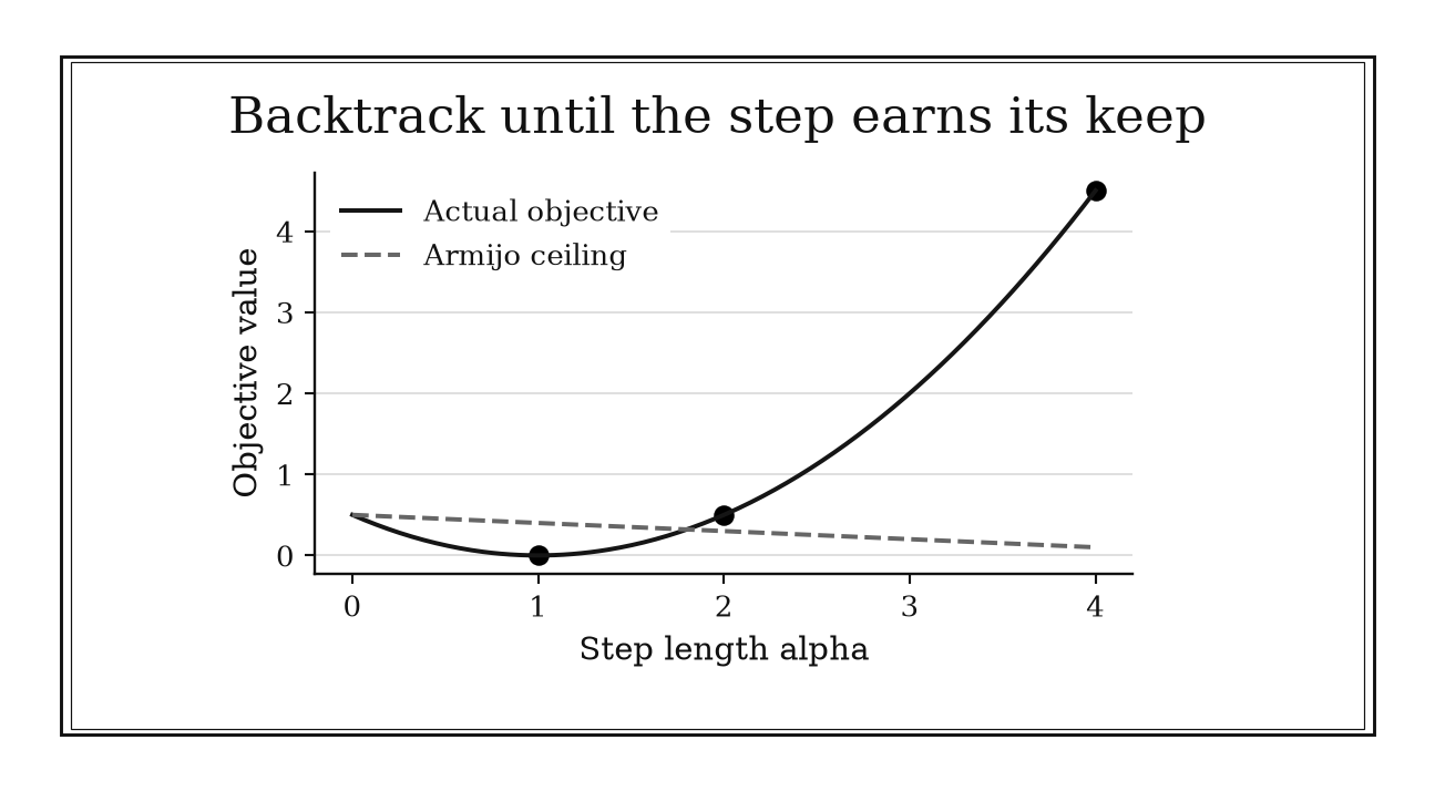
Figure 19.2. For f(x)=x²/2 at x=1 along p=-1, a trial step of four fails Armijo with c1=0.1. Halving to two still fails; halving to one reaches the minimum and passes.
19.2.3: Damp Newton until the full step is trustworthy
History
A promising fit can overshoot into nonsense the moment a full Newton step is trusted too early. Donald Marquardt built a fix for that risk in 1963, extending Kenneth Levenberg’s 1944 idea for nonlinear least-squares problems. His damping parameter interpolated between cautious descent and a fast, curvature-based Newton step, growing less conservative only as the local model proved trustworthy against the data. Modern damped Newton methods generalize that bargain beyond least squares: exploit curvature whenever available, but earn the right to take the full step.
The equation
The Newton direction solves
A globalized update is
where a line search or equivalent safeguard chooses . Near a regular minimizer, repeated acceptance of enables quadratic local convergence.
How to read it
A Newton step exactly solves the quadratic approximation built from the cost function’s curvature (its second derivative), excellent when that approximation is accurate and a wild overreach when it is not. Damping shortens the move, taking only a fraction of the full step, until actual behavior confirms the local model is reliable at that distance.
Damping controls only the step’s size, not direction: if the curvature matrix is not shaped like a genuine bowl at that point, the Newton direction may not even point downhill, and shortening the step will not fix that.
How to use it
Extreme starting coefficients push a logistic disease-risk model toward the edge where the likelihood overflows, and the raw Newton step a hospital biostatistician computes there threatens to cross it. Backtracking to produces a genuine decrease, so the biostatistician takes that step and rechecks next iterate. As coefficients settle, the full step begins passing repeatedly, signaling that fast, quadratic convergence has begun.
The rule protects against an overreaching step, not a broken direction: if the directional derivative of the Newton step is not negative, the curvature matrix is not behaving like a bowl, and damping alone will not fix it, calling for a positive-definite correction or a trust-region switch instead. This is a Workflow rule: damping is the globalization stage that connects a local Newton model to dependable progress.
19.2.4: Use the trust-region ratio to accept and resize steps
History
Whether today’s trust-region ratio is really Marquardt’s own 1963 idea, or a later formalization, is not obvious from the outset. Marquardt’s method, the safeguarded least-squares approach described earlier in this chapter, adjusted how conservative each step should be by how useful the local model had proven last try. Modern methods make the comparison explicit: divide the actual reduction by the reduction the model predicted, rather than folding it into one damping number. The ratio steers one local model; alone it never certifies the accepted point is truly optimal.
The equation
Choose a step approximately minimizing a model within
Then compute
The denominator must be positive and numerically meaningful. Acceptance and radius thresholds are algorithmic choices.
How to read it
Picture the optimizer proposing a move within a “trust region” of radius , sized to where the local model is believed honest. The ratio compares what happened to what the model predicted: near one means the model called it correctly, small and positive means overly optimistic, negative means the objective worsened. Shrinking after a bad ratio asks for a safer patch; growing it after a good ratio exploits a model that has proven itself.
The ratio cannot tell noise apart from a genuinely bad model: if the objective carries error comparable to the predicted reduction, can look bad even when the model and step were reasonable.
How to use it
A local model predicts one adjustment will cut forecasting error by 10 units for a city transportation planner’s congestion model running under trust-region control. The actual reduction is 8 units, so , high enough to accept, and since the trial reached the region’s edge, the planner widens it next round. Had the error risen by 2 units, would call for rejection and a smaller region.
The ratio is a step-acceptance rule internal to this algorithm, and is silent on whether the model itself is well specified: if sensor noise rivals the predicted reduction, healthy-looking values can still be chasing noise. This is a Specialized rule: the ratio is an internal accept-and-resize step specific to trust-region globalization.
19.2.5: Use L-BFGS when dense Hessian storage is impossible
History
How does a curvature-based search work at all on a model with ten million variables, when storing full curvature information would need more memory than any machine holds? Dong Liu and Jorge Nocedal answered a version of this in the same 1989 tests mentioned earlier in this chapter: rather than storing the whole curvature matrix, their method fit inside a fixed, small multiple of the variable count, recovering much of the benefit of curvature-aware search on far larger problems, while showing that how much history is kept, and how scaled, changes results substantially. Limited memory was never the same as memory-free or tuning-free.
The equation
For stored curvature pairs
L-BFGS uses approximately
with often in the rough range 5–20.
How to read it
A curvature-aware search builds its sense of the cost function’s shape from how the gradient, the direction of steepest increase, changes as it moves; the limited-memory version keeps only the last handful of those changes, trading a table of numbers, one entry per pair of variables, for a small multiple of the variable count.
The rule does not say how many past steps to keep: too few discard useful curvature, too many spend memory for little benefit, and no single length is best across problems.
How to use it
With parameters, a dense curvature matrix for a university learning-analytics team’s model would need roughly
far beyond the cluster. Keeping ten pairs of position-and-gradient vectors instead needs roughly
about 1.6 gigabytes, well within the largest node’s reach. The team scales the parameters first, adds a line search, and chooses a bounded variant when some parameters must stay within simple limits.
The technique assumes recent pairs reflect genuine curvature; a noisy training feed or discontinuous loss can violate the requirement that a step and its gradient change point compatibly, corrupting the curvature. The team discards any pair that fails this check. This is a Workflow rule: L-BFGS is a method-selection and memory stage inside a smooth large-scale solve.
19.2.6: Use multiple starts for nonconvex local optimization
History
A printout of final energies from repeated local searches on one atomic cluster, nearly identical except for an outlier or two sitting lower, is itself evidence the energy surface has more than one valley worth exploring. In 1997, David Wales and Jonathan Doye, working between Cambridge and Amsterdam, perturbed a cluster of Lennard-Jones-bound atoms and handed each configuration to a local minimizer. The process, run over and over, found low-energy structures for clusters of up to 110 atoms one search would likely have missed, making a common metaphor literal: one search finds the bottom of one valley, never the whole terrain.
The equation
For diverse feasible starts , compute
For maximization, reverse the final comparison. All runs must use comparable feasibility and stopping tolerances.
How to read it
A local search follows nearby slope downhill and stops at the bottom of whatever valley it starts in; it cannot climb over a ridge into a different, deeper valley. Launching many searches from varied points samples several valleys while keeping each fast, then keeps the best result found. How often a valley turns up describes the spread of starts tried, not a probability it is deepest.
Repeating a search and landing on the same answer builds confidence it is robust to small perturbations. It never turns that into a finite guarantee that no deeper valley exists unexplored.
How to use it
A delivery-routing company runs its overnight optimizer from twenty randomized starts; eighteen settle on a cost of 10.2 driver-hours while two land on a better 7.9. Since the company minimizes cost, the rare 7.9-hour result is worth deploying, and a default start would likely return only the common, worse answer. The team builds starts from randomized orderings, regional groupings, and tweaks to yesterday’s plan, then clusters routes by cost and driver-depot assignment.
Two routes assigning the same drivers to the same stops in reverse order can report identical cost while looking like separate discoveries; the team merges such duplicates before trusting the count, since counting them separately would inflate confidence beyond what the search supports. This is a Workflow rule: multistart is an exploration stage wrapped around a local optimizer, not a standalone global certificate.
19.3: Verify the Derivatives and Certify the Stop
A solver can stop because progress is small, because its derivative is wrong, or because the requested optimality conditions are genuinely satisfied. Those are different events. These rules make derivative checks economical and match stopping evidence to convex, constrained, Newton, splitting, penalty, and sensitivity settings.
19.3.1: Check gradients with directional differences, not every coordinate
History
Verifying a hand-coded gradient for a model with a million parameters is its own design problem: a poorly chosen numerical comparison can just as easily miss a bug as manufacture a false one. In June 1983, Philip Gill, Walter Murray, Michael Saunders, and Margaret Wright showed standard advice for finite-difference step sizes could give poor estimates on a badly scaled problem, balancing truncation error against the function’s scale and evaluation noise. Their paper built such gradients from scratch; checking an already-coded gradient with a few directional versions is the modern use of that balance.
The equation
For a unit direction , compare
After nondimensionalization, a centered-difference starting scale is often
where represents arithmetic or effective function-evaluation noise.
How to read it
Comparing a coded gradient against a numerical estimate along one random direction tests every parameter at once, at the cost of two evaluations, since a wrong gradient disagrees with the correct one along nearly any direction. As step size shrinks, the two should agree more closely, then level off at a plateau set by the balance of approximation error and evaluation noise.
Clean agreement on a handful of random directions does not prove every parameter’s gradient entry is correct: a bug confined to a small subset of parameters can slip through a few random checks essentially undetected in a high-dimensional model.
How to use it
A process engineer has hand-coded the gradient of a manufacturing simulation with parameters and must verify it before an overnight run. Checking every coordinate costs evaluations; five directional checks cost only , negligible against the budget. The engineer draws five random directions, adds two exercising a pressure limit and a temperature boundary, and sweeps several , watching agreement improve then level off.
A plateau at a larger-than-expected discrepancy does not, by itself, prove the gradient wrong: nonsmooth kinks or numerical noise can produce the same signature as a coding error. The engineer reruns near a known-smooth point before concluding the gradient needs fixing, treating a clean pass as a screen, not proof every entry is correct. This is a Workflow rule: directional differences are a derivative-verification guardrail before trusting search or stopping behavior.
19.3.2: Use the duality gap as a global convex certificate
History
A solver’s progress can look finished, its objective barely moving iteration to iteration, while the true gap to the best answer is still large, provable only by a second calculation bracketing the optimum from below. In December 1984, Narendra Karmarkar, working at Bell Laboratories, published a polynomial-time interior-point algorithm for linear programming, moving through a region’s interior rather than its edges. His method and its descendants made primal-dual measures, a feasible objective value alongside a companion lower bound, central to stopping, a signal exact only when both values are genuinely valid and the problem is convex, bowl-shaped with no false valleys.
The equation
For a minimization problem, let be a feasible primal value and a feasible dual lower bound. Weak duality gives
so
A relative report can scale the gap by .
How to read it
Every minimization problem has an unknown best value between two computable numbers: a feasible design’s actual cost, which can only be too high, and a “dual” quantity that can only be too low. Their difference, the duality gap, brackets how far the current design could be from the unreachable optimum, without the variables resembling the eventual answer.
A poor choice of the companion lower bound can leave a wide gap even around an excellent design. A large gap by itself only measures how loose that bound is, not how good the design is.
How to use it
An investment-allocation team has a convex portfolio problem, minimizing tracking error subject to a budget constraint, a rule limiting how the money splits, and their solver reports a feasible allocation costing 103.2 basis points alongside a companion lower bound of 103.1. Since , the allocation is within basis points of the best possible one, regardless of how different it looks from an ideal portfolio. The team sets its stopping tolerance at half a basis point.
The certificate depends on genuine feasibility of both quantities: if the allocation violates the budget constraint by a small amount, the 0.1-point gap overstates how close the truly feasible allocation is to optimal, so the team checks constraint violation before trusting the bound. This is a Workflow rule: a feasible primal-dual pair supplies the stopping certificate within a larger convex solution process.
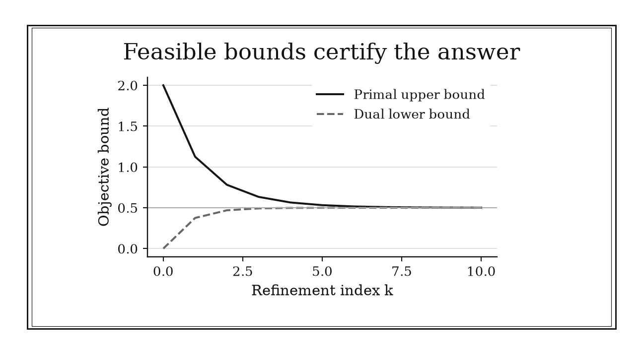
Figure 19.3. For min x²/2 subject to x>=1, primal x=1+2^-k and dual multiplier lambda=1-2^-k give valid bounds around the optimum 0.5. Their shrinking gap certifies objective accuracy.
19.3.3: Stop constrained gradient methods with a projected-gradient mapping
History
Using the raw gradient as a stopping test near a constraint boundary can leave a solver running forever, chasing a signal that never shrinks to zero even though the best answer already sits in front of it. Allen Goldstein addressed this in 1964, combining a gradient move with a projection back into the allowed region, the feasible region, whenever the unconstrained move would have wandered outside it, making the displacement from projecting, not the raw gradient alone, the signal of a constrained resting point.
The equation
For a nonempty closed convex feasible set , a feasible point , and reference step , define
where is Euclidean projection onto . A stopping condition uses a scaled form of
Feasibility should be checked separately if projection or arithmetic is approximate.
How to read it
At an unconstrained resting point the gradient, the direction of steepest increase, is exactly zero; at a constrained one it need not be, since the best direction might point out of the allowed region. The mapping steps against the gradient, projects the result onto the region if it fell outside, and measures how far that moved the point; at a genuine optimum this displacement is zero even when the raw gradient is not.
A mapping of zero certifies stationarity only for the feasible region exactly as modeled and the step used to compute it; project onto an approximate or mislabeled region and that same zero reading no longer certifies anything.
How to use it
A farmer deciding how many hundred acres, , to devote to an irrigated crop, modeled as minimizing subject to a water-rights limit of hundred acres, finds at a raw gradient of , nowhere near a resting point by the unconstrained test. Projecting the move for any positive step gives , since exceeds the limit and caps back to 1; the mapping is zero, correctly telling the farmer the boundary is already the best answer this season.
The convenience is specific to a simple cap: a region built from several rules, such as acreage limits with crop rotation, can make projection expensive, and the reasoning could break down if the region were not a simple convex cap. This is a Workflow rule: the mapping is the correct stationarity gate inside a projected-gradient procedure.
19.3.4: Scale every block of the KKT residual
History
A stationarity check can call a candidate solution optimal while a feasibility check calls it worthless, and checking both settles which verdict to trust. Harold Kuhn and Albert Tucker resolved that at the Second Berkeley Symposium in 1951, joining stationarity (no useful direction left to move), feasibility, multiplier signs, and complementarity (an inactive constraint carrying no multiplier weight) into one checklist examined piece by piece. Scaling those pieces before comparing them is a later safeguard, not part of the original conditions: without it, a raw residual reports which units and constraint are large, not which conditions fail.
The equation
For equality constraints and inequalities , representative KKT residual blocks are
with and componentwise. Dual-sign violation is another block.
How to read it
A candidate constrained solution is checked against several yardsticks, called residual blocks: does it sit at a resting point of the combined objective-and-constraint expression, does it satisfy every constraint, and does every multiplier have the correct sign and vanish wherever its constraint is not binding. All must be small, in a shared sense, before the candidate is credible.
Exact KKT conditions are sufficient for a global optimum when the differentiable objective and inequality constraints are convex and equality constraints are affine. Under a suitable constraint qualification they are necessary at a local optimum, including in nonconvex problems, where they are not sufficient. Small residuals are numerical evidence, not by themselves an objective-gap bound.
How to use it
A structural engineer’s solver reports a force residual of N against a characteristic scale of N, alongside a geometric residual of mm against a characteristic scale of mm; the larger raw value would hide a real problem in the other block. Dividing each by its own scale gives for force and for geometry: against a shared tolerance of , force passes and geometry fails by three orders of magnitude, so the engineer flags the geometric fit instead of declaring convergence.
Rescaling a constraint by a factor of 100 divides its multiplier by the same factor, so the engineer normalizes every constraint to a consistent scale before comparing multipliers; redundant constraints can make multipliers wildly unstable even while the design remains sound. This is a Workflow rule: scaled KKT blocks form a termination and reporting guardrail within constrained optimization.
19.3.5: Use the Newton decrement as a convex stopping certificate
History
A small gradient is not automatically evidence of how close the true optimum is; turning that intuition into a real guarantee takes mathematical structure beyond convexity alone. Narendra Karmarkar’s December 1984 algorithm, the interior-point method described earlier in this chapter, revived wide interest in Newton-style curvature for convex problems. The precise stopping test used today, the Newton decrement, came later, from a separate line of self-concordant analysis pinning down when a local quadratic model could bound the remaining gap: Karmarkar’s event supplies the setting, but the inequality needed that added regularity to become a certificate rather than a guess.
The equation
For a twice-differentiable convex objective with positive-definite Hessian, define
If the Newton direction satisfies
then compute without forming an inverse. If is self-concordant in the standard normalization, has minimizer , and , then
Thus is a certified stop. For small , , so is the familiar local estimate rather than a universal bound.
How to read it
The Newton decrement measures how large the gradient is once corrected by the local curvature (the second derivative), so a small decrement means the current point is near where the quadratic approximation predicts the minimum sits. Half its square is exactly the improvement that approximation predicts for one more Newton step. Under an extra condition called self-concordance, meaning curvature cannot change too abruptly, a small decrement converts into a genuine, provable bound on how far the objective sits above the true optimum.
Without that condition, the same small-decrement number is only a rough local estimate, not a certified bound.
How to use it
An operations researcher solving a self-concordant convex allocation problem with Newton’s method, after a reliable curvature-corrected solve, obtains
so the decrement is . Because the problem is genuinely self-concordant, the certified bound is
so the researcher can stop here with a guaranteed error at that scale, after checking the linear system solved cleanly and the curvature matrix was positive definite.
If the model were only ordinarily convex, that would be nothing more than a local guess, and reporting it as certified without checking self-concordance and would be unearned; the researcher falls back to KKT residuals for any constrained version instead. This is a Specialized rule: the decrement is a certified Newton stopping test only in its self-concordant local regime.
19.3.6: Balance ADMM primal and dual residuals
History
A residual imbalance in a solver’s log, one number in the primal camp and one in the dual, tells a user something a combined error measure would hide: which of two forces is winning the iteration. Stephen Boyd and colleagues connected the older alternating-direction method of multipliers to distributed statistics around 2010, splitting a problem across pieces linked by a shared constraint, and gave formulas for two residuals, one tracking feasibility and one tracking a dual-stationarity defect, recommending a penalty adjustment whenever the two sat far apart. That made balancing usable in practice, though its factor stayed a rule of thumb.
The equation
For the coupling constraint , representative ADMM residuals are
and
Here, measures primal feasibility, tracks dual stationarity change, and is the augmented-Lagrangian penalty.
How to read it
Splitting a problem into pieces linked by a shared constraint produces two error signals each iteration: a primal residual measuring how far the pieces disagree, and a dual residual measuring a stationarity defect caused by changes in the split variable. The multiplier change itself is . Increasing emphasizes feasibility in the subproblems, but neither residual is guaranteed to improve monotonically.
Adjusting to fix an imbalance is a heuristic, not a proof: nothing guarantees changing the penalty will speed convergence, only that a persistent, badly skewed imbalance is worth investigating.
How to use it
After normalizing units, a food-distribution network’s warehouse-allocation solve shows a primal residual (how much warehouses disagree on shared truck capacity) of against a dual residual (the remaining dual-stationarity defect) of . Doubling the penalty from to pushes warehouses toward agreement; under , the team rescales so the unscaled multiplier stays unchanged.
Chasing the ratio too aggressively can cause the oscillation it is meant to cure: adjusting every iteration to ordinary noise, rather than a trend, can leave both residuals swinging without converging. The team adjusts infrequently, after confirming scaling and subproblem accuracy are not the culprits. This is a Specialized rule: residual balancing is an internal penalty-control step for ADMM, not a general optimality certificate.
19.3.7: Do not make penalty parameters enormous too early
History
A penalty weight set to look practically infinite can leave a solver unable to make reliable progress, stalling the calculation it was meant to make tractable. Richard Courant, working in New York in 1943, replaced a difficult constraint in a variational problem with a finite penalty term instead, showing the true answer emerges as a limit as that weight grows without bound, a construction that also exposed a danger: the approximating problems can grow severely ill-conditioned long before finite arithmetic reaches that limit. The warning against an enormous starting weight is a modern reading, drawn from later practice, not his paper.
The equation
For equality constraints , a quadratic-penalty objective is
Its Hessian contains the term
along with second-derivative terms involving . Thus increasing simultaneously discourages violation and magnifies normal curvature.
How to read it
A quadratic penalty adds a cost proportional to times the squared violation of a constraint; a small leaves the violation visible, while an enormous crushes it toward zero but makes the problem stiff, the cost changing fast perpendicular to the constraint surface and barely along it. That mismatch is what a solver’s calculations struggle with.
The theoretical limit as describes an idealized sequence of exact solves. It is not an instruction to start the first solve near the limits of a computer’s floating-point range.
How to use it
A gym chain optimizing a weekly class-schedule with a soft penalty against any room exceeding capacity has an objective with curvature eigenvalues near 1, matching the constraint’s eigenvalue near 1. Setting the penalty to introduces curvature near , a condition number of roughly a trillion before preference terms are considered. Instead, the team solves first with , warm-starts from that schedule, raises the penalty fivefold each round, and stops successfully only once scaled constraint violations and inner-solve stationarity meet declared tolerances. If they merely stop changing above tolerance, the team investigates scaling or solver stagnation.
A lecture hall’s capacity and a small studio’s sit at different orders of magnitude, so the team normalizes each constraint before assigning a shared weight; skipping that lets one dominate for reasons unrelated to which conflict matters most. This is a Specialized rule: gradual penalty continuation is a method-specific stage inside constraint handling.
19.3.8: Read a Lagrange multiplier as marginal value
History
Assigning machines to jobs by feel can burn capacity on a factory’s worst-suited jobs while its best machines sit idle. In 1938, Leonid Kantorovich was handed this problem: allocate plywood production across machines each good at different jobs. He found more than a schedule; he found numbers attached to each machine behaving like prices, though no market had set them, calling them “resolving multipliers” in his 1939 book. His 1975 Nobel lecture linked them to Koopmans’s term “shadow prices,” values describing exchange relations near an optimal plan.
The equation
For
write with . Locally,
For minimization with ,
The sign changes when the constraint or Lagrangian is written differently.
How to read it
Each scarce resource, such as a machine’s available hours, carries a multiplier whose units are value per unit of resource, the way a price is dollars per unit of goods. A positive multiplier on a binding limit says relaxing it a little improves the result by roughly that much per unit; a resource with slack left over carries a multiplier of zero.
This reading is local: at a point where the optimal plan’s structure is about to change, a kink, the value function may bend rather than have one well-defined slope, and the multiplier there may not be unique.
How to use it
A factory manager deciding whether to lease more machine-hours for a line modeled by , with lease , finds optimal output there is ; stationarity, , gives , so each extra machine-hour is worth about 4 units of output. Leasing one-tenth more predicts a gain of , while the exact gain at is , close enough to trust the multiplier.
The price expires fast if the manager leases too much at once: once reaches 5, the unconstrained optimum at becomes reachable, the constraint goes slack, and the multiplier for further leasing drops to zero, so a price set at the current lease size cannot value a much larger lease without resolving the problem again. This is a Workflow rule: the multiplier becomes a sensitivity estimate after a valid constrained optimum has been certified.
Chapter Synthesis , Prepare, Recover, and Certify
Optimization is a sequence of claims. Scaling claims that coordinate distances and residuals represent comparable physical changes. A search step claims that local derivative information predicts useful movement. A stopping test claims that the remaining error is small in the sense the decision requires.
Prepare the first claim before tuning. Nondimensional variables and coordinate curvature prevent arbitrary units from controlling steps. Stable log-sum-exp makes sure the objective exists numerically. Condition number predicts when plain descent will be slow, while the stochastic noise-floor model prevents endless pursuit of deterministic accuracy with noisy gradients.
Make the second claim reversible. A reciprocal smoothness step is safe when is known. Armijo backtracking and damped Newton shorten overconfident moves. Trust regions test the model directly. L-BFGS preserves useful curvature when dense storage is impossible, and multiple starts reveal that one nonconvex solve samples only one basin.
Demand evidence for the final claim. Directional checks protect the derivatives. Duality gaps, projected-gradient mappings, scaled KKT blocks, and Newton decrements match different problem structures. ADMM residuals and penalty continuation diagnose algorithm internals. A multiplier becomes economically meaningful only after the constrained solution supporting it is credible.
Across all nineteen rules, ask four questions:
- Are variables, constraints, derivatives, and tolerances expressed on compatible scales?
- What observation makes an accepted step trustworthy and a rejected step recoverable?
- Which stationarity, feasibility, or global-bound condition defines completion?
- Is the conclusion local, global, stochastic, or conditional on a particular active set?
One-Page Optimization Toolkit
| Recognition cue | First calculation or action | What it gives | Role |
|---|---|---|---|
| Variables mix units or magnitudes | Set with meaningful scales | Comparable geometry and tolerances | Workflow |
| Coordinate descent sees unequal columns | Use or standardize | Coordinate step scales | Workflow |
| Exponentials may overflow | Subtract | Stable log-sum-exp or softmax | Workflow |
| Smooth strong-convex descent is slow | Estimate | Iteration-speed scale | Independent |
| Constant-step stochastic loss plateaus | Compare mean-square parameter error with | Noise-versus-bug diagnosis | Independent |
| A smoothness bound is known | Start with | Conservative gradient step | Workflow |
| Safe step is unknown | Apply Armijo backtracking | Sufficient-decrease step | Workflow |
| Newton model is useful but local | Dampen until is earned | Globalized Newton progress | Workflow |
| Model and objective may disagree | Compute actual/predicted reduction | Trust-region acceptance and radius | Specialized |
| Dense Hessian storage is impossible | Store recent pairs | Limited-memory curvature | Workflow |
| Objective is nonconvex | Launch diverse comparable local solves | Basin sensitivity | Workflow |
| High-dimensional gradient code is new | Test random directional differences | Cheap derivative verification | Workflow |
| Convex primal and dual points exist | Compute | Global objective bound | Workflow |
| Closed convex constraints alter stationarity | Compute | Projected stationarity | Workflow |
| General constrained solve stops | Scale KKT residual blocks separately | Feasibility and stationarity audit | Workflow |
| Standard self-concordant Newton solve, | Compute and | Certified objective-gap bound | Specialized |
| ADMM residuals are imbalanced | Adjust after scaling residuals | Splitting-method balance | Specialized |
| Penalty solve becomes stiff | Continue gradually in | Feasibility without immediate ill conditioning | Specialized |
| A resource bound is binding | Read its normalized multiplier locally | Marginal value estimate | Workflow |
Decision Path
- Does the problem mix units or characteristic magnitudes? Nondimensionalize variables and constraints, then transform derivatives, bounds, penalties, and reported sensitivities consistently.
- Can the objective be evaluated safely? Stabilize exponentials, logarithms, and reductions before diagnosing optimizer behavior.
- Is the objective smooth and convex? Use a reciprocal smoothness step or backtracking; use condition number to judge whether scaling, acceleration, or curvature is needed.
- Are gradients noisy? Identify the batch-variance and constant-step floor before tightening tolerances or declaring a bug.
- Is second-order information available? Globalize Newton with a line search or trust region; use L-BFGS when only a small vector history fits.
- Is the landscape nonconvex? Treat every local solve as one basin sample and escalate to global methods when a certificate matters.
- Have derivatives been independently checked? Sweep centered directional differences across several steps before trusting convergence behavior.
- What does optimality mean here? Use a duality gap for valid convex bounds, a projected mapping for closed convex sets, or full scaled KKT blocks for general constraints.
- Is the diagnostic algorithm-specific? Keep Newton decrement, ADMM balancing, and penalty continuation attached to their required method and assumptions.
- Will a multiplier drive a decision? Verify the active set, units, signs, regularity, and locality before interpreting it as marginal value.
Transfer Problems
1. A badly scaled stochastic calibration
A calibration has two variables near and , uses constant-step noisy gradients, and plateaus after 500 iterations. Design characteristic scales, transform the gradient, and explain how you would distinguish bad conditioning from a stochastic noise floor. State what should happen to transient speed, stationary mean-square parameter error, and standard-deviation width when the learning rate is halved, and identify evidence that would force a different diagnosis.
2. A Newton method that cannot decide how far to move
A smooth nonlinear objective supplies gradients and Hessian-vector products. A full Newton step predicts a reduction of 12 but raises the objective by 3; a shorter trial predicts 4 and achieves 3.2. Apply damped-Newton, Armijo, and trust-region reasoning to the two trials. Explain which ratios or directional checks you would record, when L-BFGS might be preferable, and what repeated tiny steps would make you audit.
3. Certify and interpret a constrained solution
A convex capacity-planning solve reports primal value 250.08, dual value 250.00, scaled stationarity residual , feasibility residual , and complementarity residual . Its binding capacity multiplier is 6 objective units per machine-hour. Assess the global objective certificate and KKT evidence against a residual policy. Predict a small capacity change, then list the sign, scaling, active-set, and regularity checks required before using that prediction operationally.
Where These Ideas Reappear
- Numerical methods: conditioning, stable evaluation, finite-difference error balance, and correction-based stopping determine whether an optimizer’s arithmetic is credible.
- Statistics and machine learning: feature scaling, regularization paths, stochastic noise floors, softmax, and multistart calibration recur throughout estimation and training.
- Scientific computing: profiling, memory budgets, parallel reductions, and finite precision constrain which optimization method is practical at scale.
- Control and engineering design: KKT residuals, trust regions, and shadow prices connect physical constraints with design tradeoffs and sensitivity.
- Economics and operations research: duality gaps and multipliers turn scarce resources, production limits, and allocation problems into certifiable decisions.
- Differential equations: PDE-constrained and trajectory optimization rely on adjoint derivative checks, scaled variables, and inexact Newton solves.
- Convex analysis: projected mappings, dual bounds, strong convexity, and Newton decrements are geometric forms of first- and second-order optimality.
Historical Notes and Sources
The histories separate original algorithmic contributions from later operational rules. Values such as , an L-BFGS history of 5–20 pairs, and residual-balancing factors are implementation conventions, not constants asserted by the historical authors.
- Liu and Nocedal on scaling and limited-memory BFGS: original 1989 paper; Springer record.
- Coordinate descent and standardized regularization
paths: Friedman, Hastie, and
Tibshirani’s paper;
glmnetdocumentation. - Floating-point log-sum-exp and softmax analysis: University of Edinburgh manuscript record; published paper.
- Polyak and curvature-dependent gradient convergence: early acceleration paper; Math-Net record.
- Robbins–Monro stochastic approximation: original paper; Project Euclid record.
- Armijo’s sufficient-decrease search: original 1966 paper; publisher PDF.
- Levenberg and Marquardt on safeguarded nonlinear least squares: Marquardt’s 1963 paper; Levenberg’s 1944 paper.
- Wales and Doye’s basin hopping: original 1997 paper; Oxford publication record.
- Gill and colleagues on finite-difference intervals: original SIAM paper; Stanford publication record.
- Karmarkar and interior-point geometry: original Combinatorica paper; publisher record.
- Goldstein’s projected-gradient construction: original 1964 paper; bibliographic record.
- Kuhn and Tucker’s nonlinear-programming conditions: symposium paper; Berkeley proceedings.
- Boyd and colleagues on ADMM residuals: ADMM paper and resources; Stanford reference collection.
- Courant’s penalty construction: original 1943 paper; bibliographic record.
- Kantorovich’s resolving multipliers: English translation of the 1939 work; 1975 Nobel lecture; Nobel biographical account.