Chapter 20 , Numerical Methods: Approximation You Can Trust
A linear solver reports a relative residual of . That sounds definitive until the matrix condition number is estimated at . The calculation may have solved a nearby equation exquisitely while leaving the solution uncertain at roughly the percent scale. Whether more iterations help depends on how much error comes from the incomplete solve, arithmetic, and uncertain input data.
Numerical methods become trustworthy by separating sources of error. Conditioning belongs to the mathematical problem. Stability belongs to the algorithm. Truncation belongs to discretization. Roundoff belongs to finite arithmetic. Iteration error belongs to stopping. A small diagnostic from one layer cannot certify all the others.
The nineteen rules in this chapter form three stages. The first distinguishes sensitivity from algorithm failure and chooses stable representations for sums and polynomials. The second balances truncation against roundoff and places interpolation or quadrature effort where it is useful. The third predicts refinement and root-finding behavior, then tests whether the expected regime actually appears.
The governing habit is: name every important error source, change one resolution at a time, and require the result to behave as theory predicts.
20.1: Separate Problem Difficulty From Algorithm Failure
An inaccurate answer can arise because the problem is sensitive, because the implementation magnifies error, or because a mathematically equivalent representation discards information. These five rules diagnose that distinction before more iterations or higher precision are purchased.
20.1.1: Interpret a residual through conditioning
History
A residual near zero looks like proof of success, and for years some engineers read it that way. James Wilkinson challenged the reading in 1963, publishing Rounding Errors in Algebraic Processes from his work at Britain’s National Physical Laboratory in Teddington. He separated a problem’s sensitivity to small data changes, its conditioning, from the error an algorithm itself introduces, its stability, showing that a residual, a correction, and the true forward error answer different questions.
The equation
For and computed solution , define the residual
In compatible norms, a representative first-order bound is
where when is nonsingular.
How to read it
Here is the computed answer and is the residual, the amount by which the equation fails to balance when that answer is plugged back in. Conditioning, , is a number for how much a small wobble in the data gets magnified into a larger wobble in the true answer , the way a poorly braced structure amplifies a small nudge into a large sway. The bound multiplies the residual by that magnification factor; a tiny residual alone says only that solves a nearby equation, not that it sits close to the real answer.
How to use it
Before certifying a new axle-weight limit, a consultant reviewing a vendor’s finite-element report finds a relative residual of for the stiffness system, and a condition estimate on the same matrix comes back at . Multiplying gives the permitted forward-error scale:
A relative error near one percent in the displacement field is compatible with that residual, not the sixteen-figure precision the log suggests, so the consultant treats this as a possible normwise solution-error scale and separately checks the sensitivity of the rating. Tighter iteration or refinement can reduce solve error; improved data, reformulation, or precision may be needed if input uncertainty or rounding dominates. The bound alone does not establish a percent-level uncertainty band or an irreducible floor. This is a Workflow rule: conditioning turns a residual into a forward-error diagnostic inside a broader solve-and-verify process.
20.1.2: Use backward error to distinguish stability from conditioning
History
A disappointing answer can come from a sloppy algorithm or from a problem no algorithm could satisfy, and the output alone does not say which. Wilkinson’s 1963 rounding-error analysis gave that problem a sharper question than whether an answer merely looked accurate: which nearby input, exactly, does the computed result solve? An algorithm that always answers a question close to the one asked is stable, whatever the true answer’s sensitivity to that closeness turns out to be.
The equation
For a problem and computed result , seek such that
A relative backward error is
A backward-stable algorithm typically produces in an appropriate structure and scaling, while relative forward error can behave like
How to read it
Here is the computed result and is the exact function being evaluated. Backward error asks whether some nearby input exists for which is the exact answer. If that relative change, , is tiny, on the order of the computer’s own rounding unit, the algorithm is backward stable: it has not distorted the problem by more than an ordinary rounding step. Conditioning, , measures how far that input change can push the output, so forward error scales like ; a stable method can still return few correct digits for a sensitive input.
How to use it
A power-grid state-estimation engineer runs a new sparse factorization on the network’s admittance matrix and measures a relative backward error of , near binary64’s own rounding limit, evidence the routine itself is trustworthy. A separate diagnostic puts the condition number at , since the network mixes tightly coupled substations with nearly radial feeders. Multiplying gives a possible first-order forward-error scale:
A relative error near in the estimated voltages is compatible with a perfectly stable factorization, but the product is not a proven error floor. The engineer tests refinement and, if necessary, higher precision to separate incomplete-solve and arithmetic errors from sensitivity to the input data, reporting the assumptions behind any accuracy claim and flagging the tightly coupled substations for a componentwise check, since a small normwise backward error can still hide a large relative error in one small voltage. This is a Workflow rule: backward error diagnoses algorithmic stability within a full conditioning and validation analysis.
20.1.3: Use compensated summation for long mixed-scale sums
History
A single extra variable, carried alongside a running total, is the whole invention: it remembers what plain addition just threw away. Later laboratory and standards literature traces the compensation method to Kahan’s 1965 numerical-analysis teaching materials. Ordinary floating-point addition rounds each sum to the nearest storable value, discarding the low-order part of a small term added to a larger total; Kahan’s variable estimates that loss and feeds it back into the next addition instead of repeating it.
The equation
For running sum and compensation , Kahan’s update for each term is
The sign convention for varies among descriptions; the four assignments must be kept consistent.
How to read it
Here is the running total and is the compensation, a record of the sliver each addition rounded away. Each step subtracts the compensation from the new term, adds the result into the total, then works out what got lost by comparing the new total against what was expected. Left-to-right addition without lets a long run of small terms vanish into a much larger total, the way drops of water added to a full bucket can run off unrecorded. Compensation catches most of that loss but does not turn addition into exact arithmetic; pairwise summation, building a balanced tree instead, attacks the same problem differently.
How to use it
Eight million ledger transactions, most a few dollars, sit against a running balance in the tens of millions, and a corporate treasury analyst must reconcile the year’s total. A demonstration case shows what left-to-right floating-point addition can do to a small increment:
because adding 1 to rounds straight back to ; the ledger’s own numbers are more modest in scale, but the mechanism is identical. Kahan summation does not recover the lost unit in this particular three-term order: its compensation is also rounded away before the final subtraction. It does recover the increments in a simpler test consisting of followed by ten thousand ones, where naive sequential addition loses all ten thousand. Kahan or pairwise reduction can reduce ledger accumulation error, but severe cancellation needs a checked method such as a stronger compensated sum, an exact accumulator, or higher precision. Compiler reassociation can invalidate the printed recurrence. This is a Workflow rule: compensated accumulation is a stable reduction component inside a larger numerical calculation.
20.1.4: Use Horner’s rule for polynomial evaluation
History
A calculating clerk working by hand paid for every multiplication in minutes, so a method that cut the count mattered as much as one that cut the error. On July 1, 1819, William George Horner presented such a method to the Royal Society: evaluating a polynomial by nested arithmetic that reused each partial result instead of forming every power separately. The nested form needed only as many multiplications as the polynomial’s degree, far fewer than computing each power outright, and that arrangement became the standard computational form bearing his name.
The equation
For coefficients ordered from constant to highest degree,
write
The recurrence starts with and updates for .
How to read it
Here through are the polynomial’s coefficients, the numbers multiplying each power of , ordered from the constant term to the highest power. Instead of computing , , and every higher power separately, Horner’s arrangement works from the inside out: multiply the innermost coefficient by , add the next coefficient, and repeat. Each coefficient costs one multiplication and one addition, so a degree- polynomial needs only of each, not a growing pile of separately computed powers. Fewer operations usually mean less accumulated rounding. The nested form evaluates the same coefficients; it cannot certify whether those coefficients describe the polynomial comfortably near a troublesome point.
How to use it
A simulation specialist’s flight computer represents a rocket’s calibrated thrust curve as , with a scaled time-since-ignition variable, and must evaluate it every control cycle at . Nested evaluation computes it as
using two multiplications and two additions rather than separately forming . On a flight computer with a hard cycle-time budget, that saved arithmetic across thousands of evaluations per second is a scheduling requirement, so the specialist keeps Horner’s recurrence as the baseline.
The coefficient order must stay fixed exactly as calibrated, since reversing it silently evaluates a different polynomial. If the thrust curve is later refit near a point where its coefficients nearly cancel, nested evaluation can still return a poorly conditioned value even though the arithmetic itself is backward stable; a better-centered variable or basis, a factored representation, or higher precision may help, and each should be checked against the polynomial’s input sensitivity. This is a Workflow rule: Horner’s form is the standard evaluation stage for coefficient-based polynomials.
20.1.5: Evaluate interpolating polynomials in barycentric form
History
Lagrange interpolation had a reputation it did not deserve: generations of analysts treated it as slow and fragile, a method to convert into something else before trusting it. In 2004, Jean-Paul Berrut and Lloyd Trefethen, working between Fribourg and Oxford, argued in a SIAM Review paper that the reputation had attached to the wrong culprit: the same interpolating polynomial could be evaluated quickly and stably in barycentric form, without solving a linear system or converting to monomial coefficients. The polynomial had not changed; the route used to evaluate it had.
The equation
For distinct nodes , data , and weights
the interpolating polynomial is evaluated as
Multiplying every by the same nonzero constant leaves the ratio unchanged.
How to read it
Here are the nodes, the input points where data is already known, and are weights computed once from the spacing between nodes. The formula divides one weighted sum by another; individual terms contain division by , but the ratio has the finite limit as approaches node and equals the interpolating polynomial away from the nodes. The numerator need not diverge when . Precomputing the weights lets each new evaluation use one pass over the nodes, without solving a fresh system. At a node itself the displayed terms contain division by zero, so the implementation must return directly instead.
How to use it
A forecast modeler needs an interpolated diagnostic value from three calibration points at with values , a curve behaving like over the modeled range. The scaled weights for these equally spaced nodes are . At the query point , the barycentric formula gives
matching without solving a coefficient system, cheap enough to repeat at every grid cell of a forecast run. The modeler uses closed-form weights on a Chebyshev-spaced grid and a library routine for unevenly spaced weather stations, checking the weight construction whenever the station layout changes, since raw weight products on uneven nodes can overflow even though their shared scale cancels in the final ratio. Barycentric evaluation does not repair a badly oscillating fit built from poorly chosen nodes; scattered, noisy observations still need different spacing or a piecewise model. This is a Workflow rule: barycentric form selects the stable evaluation stage after an interpolation problem has been defined.
20.2: Choose Nodes and Steps That Balance Error
Smaller steps do not guarantee better derivatives, and more evenly spaced nodes do not guarantee better interpolation. Truncation competes with roundoff, while global approximation quality depends on where information is sampled. These rules choose a useful first scale and then demand a stability check around it.
20.2.1: Use a square-root-epsilon step for forward differences
History
A derivative computed from one arbitrarily tiny step can be worse than useless, since a step small enough to tame Taylor-series error can also drown two nearly equal function values in rounding noise. Gill, Murray, Saunders, and Wright showed exactly that failure in 1983 for scaled or noisy optimization functions, choosing forward-difference intervals by balancing truncation, floating arithmetic, function scale, and noise. The square-root-epsilon step is the clean, deterministic specialization of that balance, not a universal small number safe for every black box.
The equation
The forward approximation is
Its leading truncation error is , while floating cancellation contributes a scale like . After nondimensionalization, start near
where is the relative spacing at one (about in binary64), or more generally the effective relative evaluation-noise scale. Restore units for a dimensional variable.
How to read it
Here is the small step added to , and is machine epsilon, the smallest relative gap between adjacent numbers a computer can store, about in double precision. Taking smaller reduces Taylor-series truncation error but makes two function values more nearly equal, amplifying their rounding error once divided by . Balancing against produces the square-root scale; unknown constants shift the true optimum. The formula only starts an experiment; a step sweep supplies evidence that a usable derivative plateau exists.
How to use it
Near a nitrogen rate of kilograms per hectare, an agronomist’s crop-yield simulator returns one yield number per input and must have its sensitivity estimated using only forward evaluations. For binary64, , so the step to try is
not an arbitrarily tiny guess like , which would subtract two nearly identical simulator outputs and return mostly noise. The agronomist evaluates at , , and and looks for stable derivative digits before trusting the result, scaling for each correlated input the simulator takes. If the simulator switches irrigation logic at a rainfall threshold near the tested rate, no step size restores a clean derivative there; the result is a secant sensitivity across that jump, not a true derivative. This is a Workflow rule: the square-root scale initializes a finite-difference verification or sensitivity calculation.
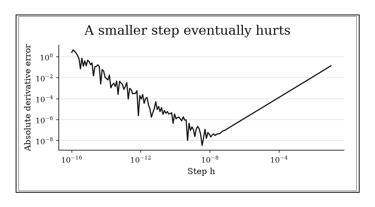
Figure 20.1. Forward differences of exp(x) at x=1 show decreasing truncation error followed by increasing cancellation error in binary64. The square-root-epsilon scale starts a sweep; it is not an exact optimum.
20.2.2: Use a cube-root-epsilon step for centered differences
History
Does a symmetric derivative formula buy an extra order of accuracy for free, or does it just relocate the same rounding tradeoff? The same Stanford group’s guidance answered the forward-difference version of that question, establishing that a difference step must balance approximation error against floating-point noise rather than chase machine precision blindly. Centering the stencil around cancels one more term of the underlying Taylor expansion, which changes the exponent in that balance, so the cube-root-epsilon rule is a later extension of their reasoning; their study focused on forward differences.
The equation
The centered approximation is
For a smooth function it has truncation and an error model
Balancing terms gives the starting scale
Here is the relative spacing at one, or an effective relative evaluation-noise scale if function values are less accurate than arithmetic.
How to read it
Here is again the small step, added on one side of and subtracted on the other, and is again machine epsilon, the smallest change a computer’s number format can register. Sampling symmetrically cancels the first-order term in the Taylor expansion, so truncation error shrinks quadratically instead of linearly as shrinks, allowing a larger optimal step than blindly chasing machine precision would suggest, since cancellation between the two sampled values still grows as they approach one another. The cube-root scaling assumes smooth, deterministic evaluations on both sides of .
How to use it
A robotics controls engineer needs a clean numerical gradient of a joint-torque model with respect to a calibration parameter near , to feed a controller-tuning routine that assumes smooth derivatives. For binary64, , so the engineer starts near
Halving and doubling that step and comparing derivative digits confirms the error balance before trusting the gradient; centered differences cost two evaluations per parameter but give a cleaner result than a one-sided formula. A friction-regime switch at a nearby calibration value defeats a centered step outright: straddling it returns a misleading blended slope that no amount of step tuning fixes, so the engineer must detect the switch and evaluate strictly on one side instead. This is a Workflow rule: the cube-root scale is a reusable component of centered numerical differentiation.
20.2.3: Use complex-step differentiation when the code is analytic
History
Every real finite-difference formula faces the same trap: shrinking the step to cut truncation error eventually forces the subtraction of two nearly identical numbers, which destroys the accuracy the small step was meant to buy. William Squire and George Trapp published an escape from that trap in 1998, perturbing a function’s input along the imaginary axis instead of the real one. Because the perturbation lives in a separate imaginary component, extracting it recovers the derivative without ever subtracting two close real values, though the trick only survives code paths that faithfully carry an imaginary perturbation through every operation.
The equation
For a real-valued analytic function extended to complex inputs,
Therefore,
with truncation and no subtraction of nearby real values.
How to read it
Here is the imaginary unit, , and is a small real step. The derivative rides entirely in the imaginary part of , while the large real value sits separately and is never subtracted from anything. Because no subtraction of two close real numbers ever happens, the usual rounding-versus-truncation tradeoff disappears, and can be made extremely small without the accuracy first improving and then collapsing the way ordinary differences do. Analytic here means every operation in the code must correctly carry that imaginary perturbation through; the formula on paper alone does not guarantee it.
How to use it
A vehicle dynamics engineer has hand-coded a gradient of a tire-force model and wants a near-exact check before trusting it in a stability controller. Testing the technique on the model’s exponential decay term, at , with a complex step :
recovering the derivative to essentially machine precision without subtracting two values near . Running the same check through the full tire-force code catches a sign error a coarser finite-difference check had missed, though the engineer still audits every absolute value, comparison, and clamp in the model, since any one of them discards the imaginary part. Where the tire model switches formulas at a slip-angle threshold, the method does not apply at all. This is a Workflow rule: complex-step is a derivative-selection and verification method conditional on an analytic implementation.
20.2.4: Use Chebyshev-like nodes for high-degree global interpolation
History
Plot a high-degree interpolant through equally spaced points and a stubborn artifact keeps appearing: oscillation piling up near the two endpoints while the middle stays calm. Herbert Salzer’s 1972 study of Lagrange interpolation highlighted practical advantages of clustering nodes near the endpoints, the cosine spacing now called Chebyshev points, where equally spaced high-degree interpolation is vulnerable to that oscillation. The pattern specifically improves the geometry of a global polynomial interpolant on one finite interval; it is not a cure for every target.
The equation
On , Chebyshev–Lobatto nodes are
Map them to by
There are nodes for a polynomial of degree at most .
How to read it
Cosine spacing crowds sample points near both endpoints and spreads them more widely near the center. This pattern controls how fast the interpolation’s worst-case amplification factor, a single number called the Lebesgue constant that measures how much small data errors can get magnified into interpolation error, grows with the number of nodes, keeping it far smaller than for equally spaced nodes at the same degree. Endpoint clustering counters the places where polynomial error tends to balloon; it does not convert extrapolation, estimating beyond the sampled interval, into interpolation.
How to use it
Free to choose where to sample rather than being stuck with fixed measurements, a graduate student running the study builds a degree-10 polynomial surrogate of a loudspeaker’s smooth frequency-response curve over its calibrated band. With , giving Chebyshev nodes, the two densest points are
showing how tightly the sampling crowds each band edge. Sampling the response at these frequencies and evaluating the surrogate barycentrically avoids the large edge oscillations equally spaced test tones would produce; the student raises the surrogate’s degree while watching out-of-sample error, not assuming more sample tones automatically help.
If a colleague hands over response data already measured on an equally spaced grid, forcing the same polynomial through those fixed points gains none of this stability; a spline or least-squares fit is the safer choice there. This is a Workflow rule: Chebyshev-like nodes select a stable sampling stage for global polynomial approximation.
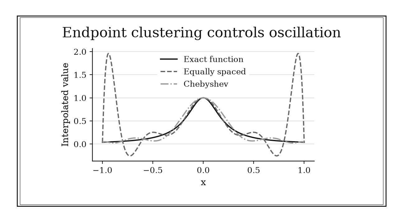
Figure 20.2. Degree-10 interpolation of 1/(1+25x²) on [-1,1] oscillates strongly with equally spaced nodes. Chebyshev-Lobatto nodes reduce this endpoint error in the constructed example; neither curve licenses extrapolation.
20.2.5: An n-point Gauss rule integrates degree 2n-1 polynomials exactly
History
Every function evaluation in a demanding integral costs real computation, so squeezing more exactness out of fewer samples is the whole game. Carl Friedrich Gauss raised the stakes on that tradeoff on September 16, 1814, presenting a new integration method in Göttingen: rather than accept fixed, equally spaced samples, he chose both nodes and weights together to obtain exceptional algebraic exactness from a limited number of function values. The modern theorem states precisely what that optimization buys for the weight and interval defining a Gaussian family.
The equation
For the relevant positive weight function , an -point Gaussian rule satisfies
for every polynomial with
The nodes are roots of the associated degree- orthogonal polynomial; the quadrature weights are not the same object as .
How to read it
Here is the number of sample points and is a polynomial’s degree, the highest power of in it. Choosing nodes as well as weights doubles the degree an -sample rule can integrate exactly compared with fixing the nodes in advance. The nodes are roots of a special family called orthogonal polynomials, whose defining property makes the quadrature’s error vanish through degree . That exactness is algebraic; accuracy for a nonpolynomial integrand still depends on how well it resembles a polynomial over the interval.
How to use it
A medical physicist computing a radiation treatment plan needs the integrated dose across a small tissue volume, where each dose evaluation requires an expensive simulation, so minimizing the sample count matters. A three-point Gauss-Legendre rule uses nodes with weights and integrates every polynomial through degree five on the normalized interval ; as a check on the smooth part of the dose profile,
recovered to rounding error from three evaluations, confirming the rule behaves as promised before trusting it on the real dose function, so the physicist uses this low-order rule inside each finite volume element instead of paying for many samples. Where the profile has a sharp edge, such as a beam boundary, three points cannot resolve it regardless of the theorem; the physicist subdivides there and compares against a nested rule before trusting the total dose. This is an Independent rule: once the Gaussian family and polynomial degree are specified, the exactness limit applies directly across quadrature settings.
20.2.6: Split adaptive quadrature where the integrand is difficult
History
An adaptive integration routine can refine its grid a hundred times over and still walk straight past a narrow spike sitting between every point it happened to sample. Robert Piessens, Elise de Doncker-Kapenga, Christoph Überhuber, and David Kahaner packaged a disciplined response to that risk in 1983 with QUADPACK: automatic one-dimensional routines that estimated local error, ranked troublesome intervals, and concentrated new evaluations where the integrand appeared difficult. The library made adaptive subdivision practical, while leaving users responsible for known singularities, discontinuities, and breakpoints that a sampled estimator might simply miss.
The equation
For known breakpoints
write
Allocate subinterval absolute-error budgets so that, conservatively,
How to read it
Here the integrand is the function being integrated, and a breakpoint is a location the user supplies in advance, marking a kink, a change of formula, or a narrow feature. Most local quadrature estimators assume the panel they are judging is smooth; a breakpoint restores that assumption by isolating the trouble spot, so adaptive refinement can spend new evaluations there instead of shrinking every panel across the whole interval. Subdivision is only as perceptive as its samples: a narrow spike sitting between every sampled location can remain completely invisible to the estimator.
How to use it
A hydrologist tests quadrature on a dimensionless pollutant-profile shape with a known kink at a plume boundary near across a normalized width of . Modeling that shape as and splitting at the kink,
turning both pieces linear and easy to integrate, whereas a blind adaptive routine would first have to discover the kink through several rounds of error-driven subdivision. The hydrologist supplies the plume boundary as a breakpoint directly, then checks the dimensionless integral against the analytic value. Actual mass discharge requires restoring concentration scale, normal velocity, and cross-sectional area through before applying a mass-balance bound. If the sampling happens to straddle a narrower secondary plume the field team has not documented, the same estimator can miss it entirely, reporting a confident total that excludes it. This is a Specialized rule: deliberate splitting is an internal quadrature stage for integrands with localized difficulty.
20.3: Budget Iterations and Verify Convergence
An advertised order is a prediction about a regime, not a badge attached permanently to a method. Refinement ratios and root brackets turn that prediction into observable evidence and evaluation budgets. These rules ask approximations to converge at the rate their smoothness and local model permit.
20.3.1: Expect a factor of four from halving trapezoid spacing
History
A single fine-mesh calculation carries an error nobody has actually measured, only assumed small. Lewis Fry Richardson refused that assumption in 1911, calculating stresses in a masonry dam on successively refined finite-difference meshes and comparing the results directly instead of trusting the finest one alone. That comparison exposed the leading discretization error and let him estimate the limiting, zero-mesh answer. For the composite trapezoid rule specifically, halving the spacing should shrink that leading error by a factor of exactly four, a specialization of Richardson’s comparison logic to one particular quadrature rule, not a claim he made for every integral.
The equation
For a sufficiently smooth nonperiodic integrand and uniform panel width ,
Therefore,
and, without knowing , successive differences satisfy
How to read it
Here is the panel width and is the trapezoid estimate at that width. Halving divides the leading error, which behaves like , by . The observed ratio of successive changes tests whether the calculation has reached the asymptotic regime, the range of fine enough spacings where that pattern actually dominates, and also estimates the remaining error from the difference itself. A ratio near four can occur accidentally once; three or more refinements make the pattern more persuasive.
How to use it
Before trusting a result for a regulatory filing, a dam safety engineer computing seepage flux under a masonry dam by trapezoid integration checks three successive mesh refinements:
The changes are 0.001 and 0.00025, whose ratio is four, matching second-order behavior. The finest result’s leading-error estimate is , small enough against the filing’s required tolerance, so the engineer submits the finest value with that conditional asymptotic error estimate stated. A sharp corner or unresolved seepage layer can spoil the expected rate, but a feature missed by every grid can also leave a misleading ratio near four. Known geometry, feature-directed refinement, or an independent calculation must support the estimate before treating it as reliable. This is a Workflow rule: factor-four behavior verifies and budgets a composite-trapezoid refinement process.
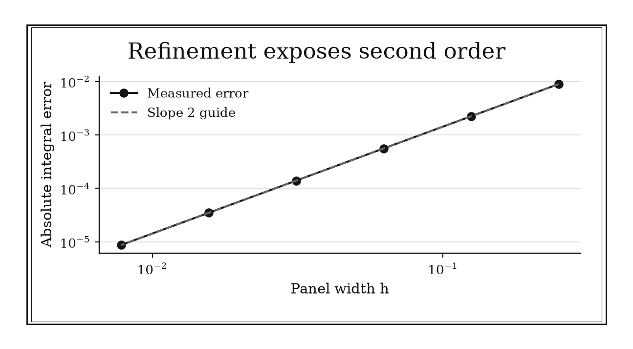
Figure 20.3. Composite trapezoid integration of exp(x) on [0,1] approaches the exact value e-1. Halving panel width reduces error by approximately four across successive refinements.
20.3.2: Expect a factor of sixteen from halving Simpson spacing
History
Does a faster-converging quadrature rule need less verification, or does its very speed make errors easier to hide? Simpson’s rule converges two full powers faster than the trapezoid rule, so its refinement signature should read sixteen, not four, when spacing is halved: the same mesh-comparison logic Richardson applied to his 1911 dam calculation, run against a rule whose error shrinks like the fourth power of the spacing instead of the second. That extra power raises the bar for convincing evidence: accidental cancellation can mimic fourth order on two meshes.
The equation
For a sufficiently smooth integrand, common endpoints, and an even number of subintervals,
Thus
and the ratio of successive computable differences also tends to .
How to read it
Here is the Simpson estimate at panel width , built from fitting a parabola across each pair of panels rather than a straight line. That symmetric, quadratic construction cancels more of the lower-order error terms than the trapezoid rule does, so halving reduces the leading error by sixteen, not four, once the asymptotic regime dominates. This faster formal rate is also easier to lose: a kink, a singular derivative, an inconsistent panel count, or unresolved oscillation can quietly prevent fourth-order behavior from appearing.
How to use it
A power-systems engineer integrates a smooth instantaneous-power waveform over one cycle by Simpson’s rule to certify a meter’s energy reading, checking three successive refinements first: , , and . The changes are
whose ratio is about 16, matching fourth-order behavior, with a finest leading-error estimate of , well below the meter’s certification tolerance. The engineer does not certify from that single ratio alone; a further refinement level confirms the pattern rather than an accidental match. A later waveform with a sharp switching transient can pull the ratio toward four instead of sixteen, and that drift itself signals the implementation has quietly dropped to lower order there. This is a Workflow rule: factor-sixteen behavior is a verification and error-budget stage for composite Simpson integration.
20.3.3: Use step halving to extrapolate away leading error
History
Two approximate answers, each wrong in a known way, can be combined into an answer more accurate than either alone. Richardson did exactly that with his mesh calculations: rather than stop at comparing spacings, he combined two of them so the leading error term dropped out algebraically, leaving an estimate of the answer at vanishing mesh size, the direct origin of Richardson extrapolation. Its power depends on an observed common error expansion; inserting a formal order without reaching that regime gives precise-looking fiction.
The equation
If
then the leading term cancels in
The correction from the fine approximation is
How to read it
Here is the approximation at resolution and is its known or verified leading error order. Both approximations, at and , contain the same unknown coefficient ; multiplying the finer result by puts its leading error on the coarser scale, so subtraction removes it algebraically. The remainder begins at a higher order only if every other error source is smaller. The correction itself doubles as an estimate of the remaining error.
How to use it
A materials consultant models peak temperature at a casting’s hot spot on two mesh resolutions, getting 0.9980 at and 0.9995 at , with order already confirmed on a third, coarser mesh. Extrapolating,
gives an estimate sharper than either mesh alone, reported alongside the correction as an error scale, having kept boundary treatment and material parameters identical across all three runs.
If the casting geometry, solver tolerance, or material model differs between mesh levels, the shared error expansion breaks and the extrapolated number becomes confident-looking fiction rather than a real improvement. This is a Workflow rule: extrapolation is an error-cancellation stage after convergence order has been verified.
20.3.4: Verify a claimed discretization order on three resolutions
History
The estimated exponent in a convergence table either matches a scheme’s advertised order or it does not: that comparison is the whole check. Richardson’s meshes turned that theoretical order into an observable quantity by comparing outputs at multiple spacings, separating the unknown limiting value from the leading power of the mesh error. The modern three-resolution check is a direct descendant, testing the code, solution regularity, and coupled tolerances together, not only the stencil written on paper.
The equation
For a constant refinement ratio
and outputs , estimate
This follows from .
How to read it
Here is the refinement ratio between successive mesh spacings and is the convergence order being estimated. Subtracting neighboring outputs removes the unknown exact value , and the ratio of those differences isolates . Three levels are the minimum needed to estimate a rate without knowing the answer; a fourth level tests whether that estimate is stable. The same norm or scalar quantity of interest must be used at every resolution.
How to use it
A CFD verification engineer checks a new solver’s advertised second-order accuracy on a manufactured test case before certifying it for a wing-design study, running three meshes at refinement ratio and getting drag outputs 1.04, 1.01, and 1.0025:
so , matching the claimed order. The engineer tightened time steps and linear-solver tolerances first so the spatial error being tested actually dominates, comparing solutions on a common representation before taking norms.
An observed order near one instead of two would suggest a coding error or an unresolved pre-asymptotic mesh, so the engineer would run a manufactured-solution study before certifying anything. This is a Workflow rule: the three-level estimate is a verification gate inside discretization and extrapolation work.
20.3.5: Budget bisection iterations from the bracket width
History
A root-finding routine that occasionally fails catastrophically is worse than one that is merely slow, since a hidden failure can reach production before anyone notices. Richard Brent addressed that stake in 1971, publishing a root finder that combined fast linear and inverse-quadratic interpolation with bisection inside a sign-changing bracket, so ordinary cases converged quickly while retained bisection supplied a worst-case guarantee close to one bit of interval reduction per fallback step. The logarithmic iteration budget is the modern explicit count behind that guarantee, and it begins only once a valid continuous sign-changing bracket has been established.
The equation
Starting from bracket , after bisections the retained width is
Its midpoint satisfies
To make the bracket width at most , budget
How to read it
Here is the bracket, an interval on which the function is continuous and its endpoint values have opposite signs, guaranteeing at least one root. Every bisection preserves whichever half still shows that sign change and discards the other half; no derivative, curvature estimate, or favorable starting point is needed, so one iteration buys exactly one binary digit of interval width. The bound controls root location, not the size of , which depends on function scale and slope.
How to use it
A bond desk quant solves a bond’s yield to maturity by bisection, representing yield in percentage points and bracketing it from 0 to 10, an initial width of 10 percentage points, with a required bracket width of percentage points. The budget is
so the pricing engine has a deterministic worst-case cost of 24 evaluations once the bracket’s endpoint signs are confirmed, a number the quant can quote to a risk committee before running anything.
The quant verifies continuity and a genuine endpoint sign change before using the budget. A root that only touches zero, such as an even-multiplicity root in a different cash-flow model, can be missed by sign-change bracketing and needs a different localization argument. This is an Independent rule: a valid bracket and requested width directly determine the worst-case bisection count.
20.3.6: Expect secant convergence of order about 1.62
History
Speed and safety trade off sharply once derivatives are gone: two nearly equal function values can turn the next step into nonsense with no warning. Brent’s 1971 algorithm managed that risk by keeping bisection in reserve while allowing superlinear interpolation steps; the plain secant method is the simplest such interpolation, a line through two recent function values with no safety net. Its golden-ratio order of about 1.618 is a local theorem for smooth simple roots, not a global promise that every step earns that many digits.
The equation
The secant update is
Near a simple smooth root, its local convergence order is
Asymptotically, for a problem-dependent .
How to read it
Here is the order, meaning error shrinks faster than a constant fraction each step but slower than squaring, a rate called superlinear. The slope through two iterates approaches the true derivative as both approach a simple root, reusing the previous function value for one new evaluation per iteration, though it lacks Newton’s quadratic rate and bisection’s containment. The order describes asymptotic error relationships, not a guaranteed reduction on each early step.
How to use it
Since the pricing model has no closed-form derivative, an actuary turns to secant iteration to find the discount rate that makes a policy’s modeled cash flows match its market price. With current error near and near one,
and the following step should reach roughly , fast enough that the actuary skips a slower bracketed method for routine pricing.
Two successive trial rates producing nearly equal modeled prices shrink the secant denominator toward zero and can launch a wild, meaningless next guess; the actuary caps the step size and falls back to bisection instead of trusting an unsafeguarded iteration. This is an Independent rule: under the simple-root local assumptions, the secant method directly carries a reusable convergence-order expectation.
20.3.7: Safeguard Newton with a bracket
History
An unsafeguarded fast root step can jump clean outside the domain it was meant to search, turning a promising method into a diverging one. Brent’s root finder never used Newton’s derivative at all, but it established the design pattern that fixes exactly that consequence: test every fast interpolation step against a sign-changing bracket and fall back to bisection whenever the step strays. A safeguarded Newton method borrows that same architecture for derivative-based steps. Brent supplied the design pattern; later engineers supplied the hybrid formula built on it.
The equation
Propose the Newton step
Accept it only if and it gives adequate progress. Otherwise use
After evaluating , replace the endpoint having the same sign so that the new bracket still contains a sign change.
How to read it
Near a simple root, Newton uses local slope information and converges quadratically, roughly doubling the correct digits each step. Far from the root, or near a small derivative, it can jump outside the domain; the bracket turns a dangerous proposal into a rejected one and preserves a deterministic route to convergence. The method trades occasional slow steps for containment; it does not make an invalid bracket valid.
How to use it
A chemical process engineer solves a reactor’s equilibrium concentration equation, modeled as bracketed on . At , and , so Newton gives
which lies inside the bracket and is accepted before updating signs. If a later near-zero derivative proposes a concentration of 20, physically impossible for this reactor, the engineer rejects it and bisects instead, requiring genuine bracket or residual progress so a useless interior step cannot stall the solver. Noisy derivatives from a stiff kinetic model may trigger repeated fallback; certification work calls for Brent’s derivative-free hybrid instead. This is a Specialized rule: safeguarding is an internal accept-or-bisect step in a bracketed Newton solver.
20.3.8: Stop Newton using the correction as well as the residual
History
A root-finding loop can look finished by one signal and unfinished by another. Wilkinson’s 1963 rounding-error analysis showed those are different claims with different failure modes: a scaled equation can make a residual tiny far from its root, while finite precision can make an update stagnate before the equation is adequately satisfied. The combined stopping rule is a modern guardrail built from that diagnostic separation.
The equation
For a scalar Newton solve, the correction is
Require both
and
where residual, absolute-step, and relative-step tolerances respect the problem’s scales. Vector problems use scaled componentwise or norm tests.
How to read it
Here is the Newton correction, the step the method proposes next. Linearization predicts , so the correction estimates remaining location error when the derivative is regular. The residual checks the defining equation directly; requiring both prevents an arbitrary equation scale or a stalled update from certifying the root alone. Neither condition proves forward accuracy near a multiple root or a singular Jacobian, the matrix of partial derivatives in several variables.
How to use it
For
the residual at is only , yet
A geophysicist inverting seismic travel-time data hits exactly this equation while solving for a velocity correction; a residual-only rule would stop at believing the velocity is found, but the correction correctly demands another step. The geophysicist chooses from the equation’s own units and from meaningful velocity accuracy, adding an iteration cap and finite-value checks. Near multiple roots, corrections can converge slowly; near singular derivatives, they can be unreliable, calling for modified Newton or a bracketed method instead. This is a Workflow rule: the dual stop is a verification gate inside a Newton root-finding process.
Chapter Synthesis: Build an Error Diagnosis Ladder
Numerical trust does not come from one tiny number. It comes from matching each diagnostic to the error source it can actually see. A residual measures how closely an equation is satisfied. Conditioning translates that residual or backward perturbation into possible forward error. Stable representations such as compensated sums, Horner nesting, and barycentric interpolation reduce avoidable arithmetic damage without changing inherent sensitivity.
Resolution choices then balance competing errors. Forward and centered differences have different optimal step exponents because their truncation orders differ. Complex-step removes subtraction but imposes analyticity. Chebyshev points control global polynomial amplification. Gaussian rules spend free nodes on exactness, while adaptive subdivision spends evaluations where smoothness fails.
Finally, convergence must appear in the output. Factors of four and sixteen reveal second- and fourth-order quadrature regimes. Richardson extrapolation is justified only after three-level refinement supports the leading power. Bisection converts a valid bracket into a deterministic budget; secant and Newton steps earn speed only under local smoothness, with bracketing and dual stopping tests protecting the calculation when that local model fails.
Across all nineteen rules, ask four questions:
- Is error caused by the problem, the algorithm, the discretization, arithmetic, or incomplete iteration?
- What scale balances truncation against evaluation and rounding error?
- Does refinement exhibit the rate the method’s assumptions predict?
- What independent residual, correction, bracket, bound, or invariant supports acceptance?
One-Page Numerical Methods Toolkit
| Recognition cue | First calculation or action | What it gives | Role |
|---|---|---|---|
| Linear solve reports a residual | Multiply scaled residual by a condition estimate | Possible forward-error scale | Workflow |
| Output is inaccurate despite a good algorithm | Compute structured backward error | Stability-versus-sensitivity diagnosis | Workflow |
| Long sum mixes magnitudes | Use compensation or pairwise reduction | Lower accumulation error | Workflow |
| Polynomial is given by coefficients | Evaluate with Horner nesting | Low-operation stable baseline | Workflow |
| Polynomial interpolant is evaluated repeatedly | Use barycentric weights | Stable interpolation evaluation | Workflow |
| One-sided derivative is required | Start with after scaling | Forward-difference step | Workflow |
| Smooth two-sided derivative is available | Start with | Centered-difference step | Workflow |
| Code is analytic and complex-capable | Use imaginary perturbation | Cancellation-free derivative check | Workflow |
| Global polynomial nodes are selectable | Use Chebyshev-like endpoint clustering | Controlled interpolation amplification | Workflow |
| Smooth weighted integral has free nodes | Use an -point Gaussian rule | Degree exactness | Independent |
| Integrand has a known kink or layer | Split and allocate local tolerances | Focused adaptive quadrature | Specialized |
| Trapezoid grid is halved | Look for change ratio near 4 | Second-order verification | Workflow |
| Simpson grid is halved | Look for change ratio near 16 | Fourth-order verification | Workflow |
| A leading error power is verified | Apply Richardson extrapolation | Canceled leading error | Workflow |
| Formal discretization order is claimed | Compare three constant-ratio resolutions | Observed order | Workflow |
| Continuous root has a sign bracket | Compute | Worst-case bisection budget | Independent |
| Derivative is unavailable near a simple root | Use secant with safeguards | Order- local expectation | Independent |
| Newton is fast but unsafe | Retain bracket and bisect bad proposals | Contained root search | Specialized |
| Newton residual alone looks small | Also test scaled correction | More defensible stop | Workflow |
Decision Path
- Does a small residual support the claimed answer? Normalize it, estimate conditioning, and check the quantity of interest before inferring forward accuracy.
- Is the algorithm itself stable? Compute a backward error in a structure and scale that represent scientifically acceptable input perturbations.
- Is arithmetic representation losing information? Use compensated reduction, Horner nesting, or barycentric interpolation before increasing precision.
- Is a numerical derivative needed? Scale the input, choose forward or centered differences from domain access, sweep nearby steps, and use complex-step only through analytic code.
- Are interpolation samples selectable? Use Chebyshev-like nodes for a global polynomial; otherwise prefer a representation suited to fixed, noisy, or nonsmooth data.
- Is an integral smooth and freely sampled? Use an appropriate Gaussian family; split at known nonsmooth locations and audit adaptive error estimates.
- Is a convergence order advertised? Run at least three resolutions with controlled coupled errors and estimate the observed rate before extrapolating.
- Is a scalar root bracketed? Budget bisection first, then permit secant or Newton acceleration without surrendering containment.
- Can a root solver stop safely? Require a meaningful residual plus location, correction, or bracket evidence, with condition checks near singular roots.
Transfer Problems
1. A small residual and an inaccurate solution
A binary64 linear solver returns relative residual for a matrix with estimated condition number . Compute the residual-based forward-error scale and explain how the algorithm could still be backward stable. Design checks that distinguish iteration error, componentwise scaling problems, and sensitivity of a particular physical output. State when higher precision would and would not help.
2. Choose differentiation, interpolation, and quadrature tools
A smooth analytic simulator accepts complex inputs on most paths, but clips one state variable at zero. It must supply a derivative, a global surrogate on , and an integral whose integrand has a known kink at 0.2. Choose among forward, centered, and complex-step differentiation; specify interpolation nodes and evaluation form; and design the quadrature split and tolerance budget. Identify the implementation tests needed before trusting each choice.
3. Verify refinement and safeguard a root
Three Simpson calculations at halved spacings are 1.500400, 1.500025, and 1.50000156. Compute the change ratio, estimate the finest leading error, and form the Richardson-extrapolated value under fourth-order behavior. A related scalar equation has a continuous sign-changing bracket of width 8 and needs width below ; budget bisection iterations and describe how secant or Newton proposals can be accepted without losing the bracket.
Where These Ideas Reappear
- Linear algebra: residuals, condition numbers, backward stability, and compensated inner products govern trustworthy factorizations and iterative solves.
- Optimization: finite-difference gradient checks, stable polynomial models, correction tests, and conditioning determine whether search and stopping diagnostics are credible.
- Scientific computing: binary precision, parallel reduction order, library behavior, and reproducibility policy shape every error budget in this chapter.
- Differential equations: Richardson extrapolation, observed order, mixed tolerances, and solver residuals recur in time and space discretization.
- Statistics and uncertainty: sensitivity, quadrature, interpolation, and stable sums affect likelihoods, expectations, bootstrap summaries, and surrogate models.
- Signal processing: polynomial filters, numerical derivatives, quadrature, and root locations appear in filter design and spectral computation.
- Engineering verification: manufactured solutions, mesh studies, independent bounds, and invariant checks turn computed outputs into auditable evidence.
Historical Notes and Sources
The historical profiles distinguish original algorithms from later operational specializations. Square- and cube-root epsilon steps, factor tests, and combined stopping tolerances are conditional error balances rather than universal constants.
- Wilkinson on rounding, backward error, residuals, and corrections: SIAM edition of Rounding Errors in Algebraic Processes; SIAM historical foreword.
- Kahan’s compensated summation: original 1965 publication; Lawrence Berkeley historical report.
- Horner’s nested polynomial computation: 1819 Royal Society paper; Carnegie Mellon scan.
- Berrut and Trefethen on barycentric interpolation: SIAM Review paper; Oxford author manuscript.
- Gill and colleagues on finite-difference intervals: original SIAM paper; journal record.
- Squire and Trapp’s complex-step method: West Virginia University repository copy; published paper.
- Salzer’s Chebyshev-point interpolation study: 1972 Computer Journal paper; Oxford Academic record.
- Gauss’s quadrature construction: Smithsonian record for the 1814 work; digitized Latin text.
- QUADPACK adaptive integration: Netlib source archive; NIST guide to QUADPACK routines.
- Richardson’s mesh refinement and extrapolation: 1911 Royal Society paper; Royal Society digitization.
- Brent’s safeguarded root finding: original 1971 Computer Journal paper; Brent’s publication archive.