Chapter 21: Scientific Computing: Precision, Performance, and Reproducibility
The same program sums the same array twice and returns two answers that differ in the last few bits. One run used four threads; the other used sixty-four. Nothing in the mathematical expression changed, yet the order of rounded additions did. The discrepancy may be harmless, or it may be the first visible symptom of a race, an unstable algorithm, or a threshold decision that amplifies microscopic changes.
Scientific computing lives at the boundary between mathematical intent and physical execution. Numbers occupy finite formats. Data move through memory hierarchies. Parallel work changes evaluation order. Long calculations encounter hardware failures. A credible result therefore needs more than correct equations: it needs explicit contracts for accuracy, comparison, reproducibility, performance, and recovery.
The eight rules in this chapter form three layers. The first budgets finite precision and protects delicate elementary expressions. The second defines reproducible comparisons and directs optimization effort toward measured costs. The third identifies hardware ceilings and balances useful computation against parallel and failure overhead.
The governing habit is: state what must be accurate, repeatable, fast, and recoverable before choosing an implementation.
21.1: Spend a Finite Precision Budget Deliberately
Floating-point arithmetic is not vague arithmetic. Its format gives a precise local rounding scale, but conditioning and algorithm design determine how that scale reaches an answer. These two rules turn binary64 precision and near-zero elementary functions into practical error-budget decisions.
21.1.1: Budget binary64 as about sixteen decimal digits
History
A single specification, hashed out over years among hardware designers and numerical analysts, decided how every conforming machine would store a number. IEEE Standard 754, adopted 21 March 1985 in the United States, fixed interoperable formats, rounding behavior, and exception handling that machines had previously disagreed about. Binary64, its double-precision format, allots a number 53 bits of significand, an engineering choice, not a law of arithmetic. That allotment produces the familiar sixteen-decimal-digit rule. The standard fixed representation and rounding, not whether those digits survive an ill-conditioned calculation.
The equation
For rounding to nearest in binary64, the unit roundoff is
The distance from 1 to the next larger binary64 number is
Since , the significand carries roughly sixteen decimal digits.
How to read it
For a finite normal result without overflow, a basic operation rounded to nearest has relative rounding error at most about , roughly one second against three hundred million years. A single rounding barely matters. A calculation’s condition number measures how much a problem stretches small input wobbles into larger output ones, so is a first worst-case sensitivity scale for a stable calculation, not a guaranteed error or floor; accumulated rounding and an unstable sequence of steps can lose still more. This budget sizes one rounded step, not a finished calculation; step count and conditioning can spend it first. Two epsilon values circulate because unit roundoff is half the gap between 1 and its next neighbor.
How to use it
A climate-model operator validating a new ocean-circulation solver needs a realistic convergence tolerance before a production run. Diagnostics put the linear system’s condition number at , so
That suggests a worst-case budget near eight digits under the assumed stable computation, rather than a guaranteed sixteen. It is not a proven accuracy floor or a residual stopping tolerance: the operator checks input uncertainty, residual-to-output sensitivity, and refinement before choosing a target. A tighter solve can help until arithmetic or input error dominates. If the solver’s inner loop subtracts two nearly equal heat fluxes every timestep, cancellation can erode digits faster than predicts, and no looser tolerance recovers them; reformulating the flux difference is the fix. This is an Independent rule: binary64’s format directly supplies a portable first precision budget, provided conditioning and accumulated error are assessed separately.
21.1.2: Use log1p and expm1 for small arguments
History
Whether a risk model treats a disaster as rare or as impossible can
hinge on a probability so small that ordinary arithmetic erases it. Sun
Microsystems confronted that risk in 1993, releasing fdlibm, a freely
distributable C library for consistent elementary-function results
across IEEE-754 systems. Its log1p and expm1
routines used range reduction and special near-zero formulas instead of
textbook expressions, preserving digits straightforward evaluation would
discard. Forming
can round straight back to 1 when
is small, hiding it from a logarithm, and the reverse cancellation
strikes
near zero. Two equivalent expressions can carry very different amounts
of floating-point information.
The equation
For small ,
and
Use the specialized evaluations
when forming or subtracting 1 would discard significant low-order bits.
How to read it
When
is very small,
can round to exactly 1, so an ordinary
can return 0 even though
was never zero, like a grain of sand added to a beach and lost in the
next weighing. The same erasure happens in reverse for
,
since
sits close to 1 and subtracting 1 cancels the digits that mattered.
log1p and expm1 reorganize the arithmetic so
the small result is computed directly, without forming the near-1
intermediate that would swallow it. What this does not fix:
log1p(x) still requires
;
a stable evaluator makes a calculation trustworthy, not an invalid input
valid.
How to use it
A catastrophe-risk analyst estimates the probability of at least one damaging storm occurring in a given second, using with a dimensionless one-second event exposure . In binary64 arithmetic rounded to nearest, the naive calculation gives
since rounds to exactly 1 before the subtraction runs, reporting the storm as impossible. Routed through the stable identity instead,
the true nonzero probability the decision depends on. The analyst carries that stable form through the pricing formula, since rebuilding any intermediate step from the naive expression reintroduces the cancellation. No stable routine makes a negative event exposure valid; this probability model requires . This is an Independent rule: whenever a legitimate small argument creates cancellation in these two standard forms, the specialized functions are reusable replacements.
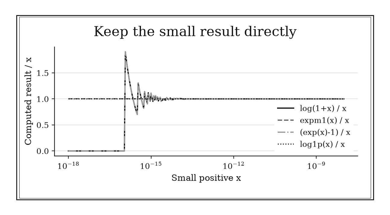
Figure 21.1. The ratios log1p(x)/x and expm1(x)/x stay near one for tiny positive x. Forming log(1+x) or exp(x)-1 first can lose most or all of the result to rounding.
21.2: Make Reproducibility an Explicit Contract
Reproducibility has levels. A result may agree scientifically within a tolerance, numerically to several digits, or bit for bit. The correct requirement depends on the decision the computation supports. These rules define comparison policy and ensure that performance work begins with evidence rather than intuition.
21.2.1: Expect parallel floating reductions to change low bits
History
Two runs of the same parallel sum, on different thread counts, can return different answers though nothing about the underlying mathematics changed. In 2016, Berkeley researchers James Demmel, Willow Ahrens, and Hong Diep Nguyen traced that failure to its source: dynamic parallel reduction order combined with nonassociative floating-point addition. They designed a compact accumulator and ReproBLAS routines that return bitwise-identical sums regardless of scheduling, making the guarantee’s accuracy and performance cost explicit. Their finding reframed a class of bug reports: a changed last bit can be harmless rounding, but confirming that requires a declared policy on acceptable variation.
The equation
Rounded addition is generally nonassociative:
where denotes floating-point rounding.
Different reduction trees evaluate different parenthesizations of
How to read it
Real-number addition does not care what order you add things in, but floating-point addition does, because every intermediate sum gets rounded to the nearest storable value before the next term is added, like rounding a running total to the nearest cent after each item rather than only at the end. Changing thread count, scheduling, or compiler regrouping can change which small terms get rounded away first, altering a sum’s last few bits with no data race involved. Those shifted bits are usually harmless alone, but an iterative or threshold-driven calculation can amplify them. This rule tells you such variation is expected; it does not tell you how large an acceptable variation is for your decision.
How to use it
A genomics pipeline analyst reruns a variant-calling job on 8 and then 64 threads and finds the read-depth sum disagrees in its last few digits. A toy triple shows the mechanism: with , , , one grouping gives
while can give 0, since rounds straight back to before is added. The real discrepancy is a relative difference of , over the variant-calling decision margin of . After independently checking synchronization and excluding races and undefined behavior, the team adopts a deterministic reduction tree, recording compiler, thread count, and library version. This is an Independent rule: order-dependent rounding directly predicts possible low-bit variation across parallel reductions, independent of any particular programming language.
21.2.2: Compare floating results with absolute plus relative tolerance
History
An automated equality check can fail for numbers that are effectively
identical, and pass for numbers nowhere near each other: both are
consequences of comparing floating-point results the wrong way. Python’s
community confronted that in 2015 through PEP 485, an international
proposal on approximate equality across many magnitudes. It documented
why a fixed small absolute tolerance can reject acceptable relative
differences at large magnitudes and why a purely relative tolerance
fails near zero (agreement to a fraction of nothing). The accepted
design exposed separate relative and absolute controls in
math.isclose, standardizing a pattern, not a choice of
tolerances. That API takes the maximum of its absolute and relative
allowances; the equation below is a common additive alternative.
The equation
A common symmetric comparison accepts and when
Here, atol supplies a floor near zero and
rtol permits error proportional to magnitude away from
zero.
How to read it
A comparison test has two knobs. The relative tolerance,
rtol, allows error that grows with the size of the numbers,
like a tailor allowing a wider margin on a tent pole than a shirt cuff.
The absolute tolerance, atol, sets a fixed floor for small
numbers, so the test does not demand perfection near zero. The test
accepts
and
when their difference is no larger than atol plus
rtol times the larger magnitude. If both values are tiny,
the floor does the work; if either is large, the relative term takes
over. Passing this test means the numbers are close enough, not that
either is correct.
How to use it
A semiconductor test engineer compares a simulated output voltage against a bench reading to decide whether a chip passes. Simulation reports microvolts, the bench reads microvolts, a relative difference of
comfortably inside a chosen rtol of
.
Elsewhere, a leakage-current channel reports 0 in simulation against a
measured
amps; relative tolerance is meaningless there, so atol, set
from instrument noise floor, governs instead. rtol comes
from simulator discretization error, atol from meter
resolution, not whatever number makes a test pass. Across thousands of
channels, the engineer checks per-channel results rather than one
aggregate norm, which can hide a drifting channel. This is a
Workflow rule: the mixed tolerance is a reusable gate
inside a broader verification and regression-testing process.
21.2.3: Profile before optimizing scientific code
History
Which part of a program is slow? Presumption and behavior disagree, and routine-level timing alone can hide the cost inherited from called routines. Susan Graham, Peter Kessler, and Marshall McKusick, at Berkeley, published gprof in 1982 to test presumption against measurement: sampled execution time combined with call-graph counts, tracing cost through a function and everyone calling it. A programmer could see how execution costs propagated through the calling structure before rewriting anything. The tool made hot-path measurement practical, but its numbers stay specific to one build, input, machine, and run.
The equation
If a component occupies fraction of total runtime and is accelerated by factor , the new normalized runtime is
so the fractional saving is
How to read it
Total runtime is a weighted sum of every part of a program, and a profiler estimates how much each part occupies, like trimming a grocery bill that is 2% of household spending instead of the rent. That fraction reveals whether time belongs to arithmetic, memory allocation, input and output, synchronization, or a function that looks innocent but is called constantly from elsewhere. Even a spectacular speedup on a small fraction cannot move the total much, while a modest speedup on a large fraction can. A profile shows where time is going; it does not tell you which fix works.
How to use it
A game studio build engineer must speed up a stalling frame-render pipeline before a milestone, and the team’s first instinct is to hand-optimize a physics-collision routine remembered as slow last year. Profiling the shipping build shows that routine now occupies only 5% of frame time; even a 100-fold rewrite saves at most
under 5%. The same profile flags an asset-streaming step at 70%; halving that cost would save
or 35%, seven times more. The engineer redirects toward streaming, profiling a release build on a representative level rather than the debug scene the hunch was based on, since cold caches and profiler overhead there can distort a cost either way. This is a Workflow rule: measurement selects and verifies each performance intervention inside an iterative optimization process.
21.3: Model Hardware Limits and Failure Costs
Fast code is constrained by more than peak arithmetic throughput. Data movement can dominate arithmetic, serial work can dominate parallel work, and checkpoint overhead competes with recomputation after failure. These three models expose the relevant ceiling before expensive engineering begins.
21.3.1: Know whether a kernel is compute-bound or bandwidth-bound
History
Adding faster arithmetic units to a chip does nothing for a program waiting on memory, a mismatch once diagnosed mostly by guesswork. In 2009, Samuel Williams, Andrew Waterman, and David Patterson, at Berkeley, introduced the Roofline model: a plot placing a flat compute ceiling above a sloped bandwidth ceiling, with arithmetic intensity deciding which one constrained a kernel. The plot gave programmers a resource diagnosis before touching code. That ceiling shifts with memory level, precision, and implementation, so a kernel sits differently on different hardware.
The equation
Arithmetic intensity is
The basic Roofline bound is
where is attainable FLOP/s, the compute ceiling, and measured memory bandwidth.
How to read it
Arithmetic intensity counts useful floating-point operations per byte moved through memory. At low intensity, performance rises through data reuse, like a kitchen with idle chefs that cannot cook faster if one delivery truck limits how fast vegetables arrive; at high intensity, the chefs become the limit, and performance nears the peak compute ceiling. The crossover sits near the ratio of peak compute rate to bandwidth: below it, more arithmetic hardware buys almost nothing, since delivery is the bottleneck. What the model misses: latency, irregular access, and synchronization can hold performance below both ceilings.
How to use it
An aerospace CFD engineer must decide whether to fund a faster GPU or restructure memory access for a kernel adding two neighboring cell values. Each addition reads two 8-byte numbers and writes one 8-byte result while performing about one operation, so intensity is roughly
deep in bandwidth-bound territory. A GPU with double the peak FLOP rate would barely change runtime, since bandwidth, not throughput, is the limit, so the engineer prioritizes loop fusion and cache blocking instead. A matrix-assembly routine in the same solver reuses each value many times, giving higher intensity. For that routine, the engineer compares measured throughput, transfer costs, and both machines’ ceilings before deciding whether the GPU purchase helps. Source-level counts miss cache effects, so bandwidth gets measured directly. This is a Workflow rule: arithmetic intensity selects the likely performance strategy inside a measured tuning process.
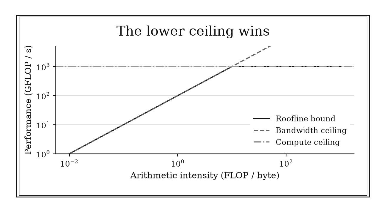
Figure 21.2. For a constructed machine with 100 GB/s bandwidth and 1000 GFLOP/s peak, the roofline bends at 10 FLOP/byte. Below that point bandwidth is the model’s limit; above it peak compute is.
21.3.2: Use Amdahl’s law to bound strong scaling
History
Just a few pages long, one conference paper punctured the enthusiasm around massively parallel machines before most were built. At the AFIPS Spring Joint Computer Conference, held 18 to 20 April 1967 in Atlantic City, Gene Amdahl argued that the portion of a fixed workload that cannot be parallelized eventually dominates execution time no matter how many processors join. The paper turned a hardware sales pitch into a bound: however fast the parallel part becomes, the serial fraction caps total speedup. Communication and imbalance typically make scaling worse, while growing the problem calls for a different model.
The equation
If fraction of one-processor runtime is effectively serial, idealized speedup on processors is
Therefore,
Parallel efficiency is .
How to read it
Picture a workload as two pieces: a fraction split across processors and a fraction that cannot be, like a relay race with a fixed baton-pass time no number of runners can shrink. Adding processors keeps shrinking the parallel piece’s share of total time, but the serial piece stays the same size, so once parallel time becomes small, more processors barely move the total. The serial fraction should include synchronization and setup costs that also refuse to shrink, not only sequential code. This describes strong scaling, fixed work spread across more processors; it leaves untouched a problem that grows alongside the machine.
How to use it
A national laboratory’s allocation committee is deciding whether to fund a fourfold cluster expansion for a fixed astrophysics workload with serial fraction . Even with infinitely many processors, speedup cannot exceed . At the proposed size of , idealized speedup is
only , or 24% efficiency, well short of a naive 64-fold gain. The committee asks for runtime at several processor counts to fit the serial fraction before approving hardware. The bound assumes fixed workload size; larger simulations on the same cluster fall under a weak-scaling model instead, where the same fraction may not even apply. This is an Independent rule: a credible fixed-work serial fraction directly bounds strong-scaling speedup across parallel systems.
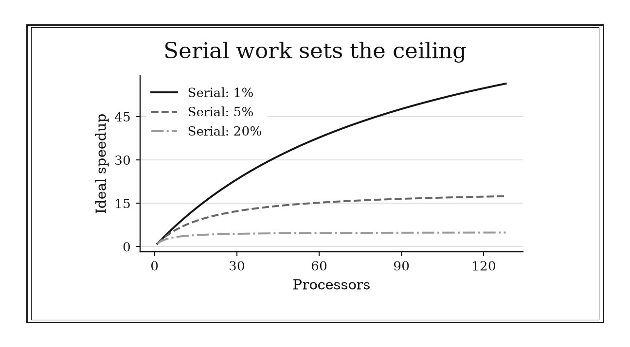
Figure 21.3. Ideal strong scaling with a five-percent serial fraction cannot exceed twentyfold speedup. The curves omit communication costs that grow with processor count, so real performance may be lower.
21.3.3: Set checkpoint interval from checkpoint cost and failure rate
History
A long calculation that checkpoints too rarely can lose days of work to one failure; checkpointing too often wastes nearly as much time writing state nobody needs. In September 1974, John Young modeled that tradeoff: runtime spent writing checkpoints against recomputation lost to failures between them. Minimizing that first-order model produced a checkpoint interval that scales as a square root, not linearly, in checkpoint cost and failure spacing. Later work refined Young’s calculation with restart costs he had not modeled, but his balance remains a practical estimate today.
The equation
Let be checkpoint duration, the mean time between independent failures, and the interval of useful work between checkpoints. The first-order waste rate is approximately
Minimizing gives
All three quantities must use the same time units.
How to read it
Picture two kinds of waste competing, like insuring a shipment daily, costing more in premiums than the rare loss it guards against, versus insuring yearly, leaving too much exposed in between. A checkpoint takes time from useful computation, and that waste shrinks the longer you wait between checkpoints. But waiting longer also means a random failure destroys, on average, about half of whatever work happened since the last one. Balancing those trends gives a square-root relationship: doubling checkpoint cost, or the time between failures, does not double the best interval, only multiplies it by about 1.4. This is a model of overhead trading, not a prediction of when the next failure strikes.
How to use it
A weather-forecast operations center running a 256-node ensemble overnight needs a checkpoint policy. Checkpoint time is minutes and mean time between failures across those nodes is minutes, so
The team sets checkpoints roughly every hour, not the 15 minutes an old single-node policy specified, since that shorter interval wastes more time than it saves. The team adds restart time and storage contention to the estimate, and rechecks for the full allocation, since more nodes fail more often than one alone. A checkpoint that cannot be restored is not protection, so recovery gets tested first. This is an Independent rule: under the periodic independent-failure model, cost and mean failure spacing directly produce a reusable first checkpoint interval.
Chapter Synthesis: Treat Computation as a Contract
Scientific computation is trustworthy when its promises are explicit. Binary64 supplies a finite representation budget, but conditioning and algorithm choice decide how much reaches the answer. Stable elementary functions protect information that a naive algebraic form would discard before useful work begins.
Reproducibility then requires a declared level. Parallel reductions may legitimately change low bits, while a combined absolute-relative tolerance states which changes are acceptable for a decision. Profiling prevents performance work from becoming folklore: measure the complete workload, intervene at a real bottleneck, protect numerical behavior, and measure again.
Performance and resilience are also modeling problems. Arithmetic intensity distinguishes data-motion limits from compute limits. Amdahl’s law exposes the fixed-work ceiling imposed by serial effort. Young’s checkpoint balance prices the opposing costs of saving too often and recovering too much lost work.
Across all eight rules, ask four questions:
- What accuracy is physically and numerically meaningful?
- Must reruns agree scientifically, numerically, or bit for bit?
- Which measured resource actually limits time to solution?
- How much completed work can the system afford to lose?
One-Page Scientific Computing Toolkit
| Recognition cue | First calculation or action | What it gives | Role |
|---|---|---|---|
| A binary64 accuracy claim | Start from , then multiply by conditioning | First precision budget | Independent |
| or with small | Use log1p or expm1 |
Cancellation-resistant evaluation | Independent |
| Parallel sum changes across runs | Inspect reduction order and error scale | Reproducibility diagnosis | Independent |
| Floating results need comparison | Set atol plus rtol from the error
budget |
Decision-aware equality test | Workflow |
| Code needs acceleration | Profile a representative release workload | Evidence-backed optimization target | Workflow |
| Kernel performance is low | Compute FLOPs per byte and compare roofs | Bandwidth-versus-compute diagnosis | Workflow |
| More processors are proposed | Evaluate | Strong-scaling ceiling | Independent |
| A long run can fail | Start with | Checkpoint interval estimate | Independent |
Decision Path
- Is the claimed accuracy close to machine precision?
Combine unit roundoff with conditioning and algorithmic error; do not
equate
epswith final accuracy. - Does an expression subtract nearly equal values?
Search for a stable equivalent such as
log1p,expm1, compensated summation, or a scaled formulation. - Do parallel runs differ? Quantify the discrepancy, rule out races and undefined behavior, then choose a tolerance, deterministic tree, or reproducible accumulator consistent with the contract.
- Are tests flaky? Derive absolute and relative tolerances from expected error and units, including explicit policies for nonfinite values and arrays.
- Is the program too slow? Profile the complete representative workload before changing code, then reprofile after each intervention.
- Is a hot kernel limited by arithmetic or data motion? Measure arithmetic intensity and hardware ceilings before choosing vectorization, blocking, fusion, or traffic reduction.
- Will more processors help? Measure strong scaling and use the effective serial fraction to bound the gain.
- Can the run outlive reliable hardware? Estimate checkpoint cost and job-level failure spacing, calculate a starting interval, and test actual restart.
Transfer Problems
1. Precision and reproducibility in a parallel sum
A parallel program sums values spanning sixteen orders of magnitude. Runs on 8 and 64 threads differ by relative, while the downstream decision changes when the sum crosses a threshold only away. Explain why reduction order matters, why the observed difference cannot simply be dismissed, and how you would separate harmless rounding from a race. Propose an accumulation method, comparison policy, and reproducibility level.
2. Diagnose a disappointing optimization
A simulation spends 70% of wall time moving data through a kernel with arithmetic intensity FLOP/byte, 20% in serial setup, and 10% elsewhere. A developer proposes doubling processor count and hand-optimizing a routine that occupies 2% of runtime. Use profiling arithmetic, the Roofline idea, and Amdahl’s law to rank the interventions. State which measurements are still needed before estimating an actual speedup.
3. Protect a long-running calculation
A 256-node job takes six minutes to write a checkpoint and has an observed job-level mean time between failures of 1,200 minutes. Compute Young’s starting checkpoint interval. Then design a policy that accounts for restart time, shared-filesystem contention, correlated outages, and validation of restored state. Explain how changing to 1,024 nodes could alter the failure model even if node reliability is unchanged.
Where These Ideas Reappear
- Numerical methods: conditioning, backward stability, compensated summation, and stopping tolerances determine how the binary64 budget reaches a computed answer.
- Optimization: stable log-sum-exp, scaled residuals, profiling, and parallel reductions affect objective values, gradients, and termination decisions.
- Statistics and simulation: random-number streams, reduction order, tolerance policy, and checkpoint recovery shape reproducible Monte Carlo evidence.
- Linear algebra: arithmetic intensity and data reuse explain why dense matrix multiplication and sparse matrix-vector products behave differently on the same hardware.
- Differential equations: mixed tolerances, precision limits, and checkpointing govern long time integrations and large discretized systems.
- Software engineering: regression tests, environment capture, profiling, and recovery drills turn numerical intent into an auditable computational artifact.
- Distributed systems: Amdahl ceilings, synchronization, failure rates, and replicated state connect high-performance computation to service reliability.
Historical Notes and Sources
The histories distinguish standards, algorithms, diagnostic models, and modern operational uses. Their numerical thresholds remain attached to the stated format, workload, hardware, and failure assumptions.
- IEEE 754 and binary64: IEEE 754-1985 standards record; IEEE Milestone history.
- Sun fdlibm and stable elementary functions: Netlib fdlibm archive; original
log1psource and method comments. - Reproducible parallel summation: Berkeley ReproBLAS technical report; SIAM project account.
- Mixed floating-point tolerance: PEP 485; Python
math.isclosedocumentation. - Measured program profiling: original
gprofpaper; historical Berkeley source and documentation. - The Roofline performance model: Lawrence Berkeley/DOE report; UC Berkeley publication record.
- Amdahl’s strong-scaling bound: original 1967 AFIPS paper; Carnegie Mellon scan.
- Young’s checkpoint interval: original Communications of the ACM paper; SIAM extension and analysis.