Chapter 22: Ordinary Differential Equations: Choosing and Checking Time Integrators
A solution curve can look smooth while the solver takes a million unnecessary steps. That is one signature danger of ordinary differential equations: a numerical method responds not only to the plotted solution, but also to fast-decaying modes, oscillatory structure, event surfaces, and scales hidden among the state variables.
ODE integration is therefore a matching problem before it is an accuracy problem. Explicit and implicit methods pay different costs for stability. Symplectic methods preserve a different kind of information than ordinary adaptive solvers. Local error estimates govern individual steps, but they do not by themselves certify long trajectories, conserved quantities, or correctly located events.
The twelve rules in this chapter form three themes. The first matches integrators to stiffness, dissipation, Hamiltonian structure, order, and frequency content. The second turns tolerances and event functions into reliable adaptive behavior. The third checks stability, convergence, invariants, and sparse linear algebra independently of a solver’s success flag.
The governing habit is: classify the dynamics, scale the error, and verify the trajectory with evidence the integrator did not use to accept its own steps.
22.1: Match the Integrator to the Dynamics
Method names are less important than the numerical obstacle. A decayed fast mode creates a stability restriction; a Hamiltonian orbit rewards geometric preservation; an oscillation demands phase resolution even when a method remains stable. Diagnose that obstacle before tuning tolerances.
22.1.1: Suspect stiffness when stability, not accuracy, dictates tiny steps
History
A numerical integrator can grind through a million tiny steps while the plotted curve barely moves, with nothing in the plot explaining why. In March 1983, in Livermore, California, Linda Petzold published a scheme reading a solver’s recent steps to decide, mid-run, whether a problem still needed a nonstiff formula or had turned stiff enough for an implicit one. Tested inside a modified LSODE package, the logic tracked a problem whose character changed as it ran. The heuristic carries its own bookkeeping cost, but it caught the moment tiny steps stopped resolving the solution and started serving stability alone.
The equation
Let a rapidly decaying Jacobian mode have eigenvalue ({fast}), with ({fast}<0). A practical stiffness signal is
while an explicit method still requires (h|_{fast}|=O(1)) for stability.
How to read it
Picture two clocks inside one system: one ticks in microseconds, one in seconds. The fast clock is a rapidly decaying piece of the solution, described by a rate called an eigenvalue: a larger negative number means faster decay. Stiffness means the step size, the gap between calculations, stays tiny after that fast piece has died out, because stability rather than accuracy demands it. A method’s stability region is the range of step sizes it can take without blowing up; an A-stable method never blows up on any decaying mode, and an L-stable one drives that mode toward zero.
The rule flags the real obstacle. It does not price the fix: nonlinear solves that can outweigh the steps replaced on a small, nonstiff problem.
How to use it
A wastewater treatment plant operator is modeling the contact tank’s disinfection chemistry before an unattended overnight run: a fast quenching step decaying on a timescale of s against a slow byproduct buildup over s, tracked out to s. Reading the fast decay as an eigenvalue, , an explicit method’s stability limit near s forces roughly steps for a transient finishing almost immediately. Watching rejected steps pile up, the operator switches to a BDF or Radau solver, advancing instead in steps set by the slow chemistry.
The switch is not free: implicit steps carry nonlinear solves, and a rapidly pulsing influent pump is not stiffness and still needs small steps. This is a Workflow rule: it selects a method from evidence about the active stability restriction.
22.1.2: Use BDF for large dissipative stiff systems
History
Left to a naive explicit method, a reaction finishing in a heartbeat can force every later step of a simulation to creep forward at that same pace, long after the fast species has vanished. In March 1952, working at the University of Wisconsin in Madison, Charles Curtiss and Joseph Hirschfelder studied stiff chemical-kinetics equations whose rapidly decaying modes were defeating explicit integration. Their fix evaluated a backward-difference formula implicitly, at the new time step, letting the calculation advance in steps sized for the slow chemistry. That paper is the direct ancestor of the BDF methods, built around dissipative stiffness as their target, not as a universal replacement.
The equation
A (q)-step BDF formula has the form
Because (y_{n+1}) appears inside (f), each step requires a nonlinear solve, normally supported by a Jacobian or Jacobian approximation.
How to read it
BDF fits a short polynomial through recent solution values, then forces its slope to match the differential equation at an endpoint it must solve for, which is what “implicit” means. The first two BDF orders are A-stable, never blowing up on any decaying mode, so the step size can be set by how fast the slow part of the system changes rather than by the fastest decaying piece. Higher orders keep useful stability but not that full guarantee, and using past values means the method starts slowly after a sharp change or restart.
How to use it
Temperature diffusion through a stack of steel ingots is being simulated by a heat-treatment furnace operator planning a one-hour anneal, s. The finest grid cell carries an eigenvalue near , so an explicit stability limit near s would require roughly steps, a run no schedule can wait for. Switching to a variable-order BDF solver, the operator instead chooses steps sized by the changing ingot temperature, say s, giving a workable steps.
That gain assumes Newton iterations converge cheaply; strongly nonlinear radiation terms can erode BDF’s speed advantage. The operator watches iteration counts alongside accepted steps before trusting the schedule. Oscillatory, lightly damped modes are a poor match for the same reason BDF favors decay. This is a Workflow rule: it chooses a stiff integration family for a recognizable dissipative regime.
22.1.3: Use symplectic integrators for long Hamiltonian trajectories
History
For a while, a numerical integrator’s formal order, how fast its one-step error shrinks on paper, was treated as nearly the whole argument for choosing it, even for trajectories meant to run for years. In 1983, working at Brookhaven National Laboratory in New York, Ronald Ruth published an explicit method built to preserve the canonical symplectic structure of Hamiltonian systems: the geometric relationship linking position and momentum that the physics respects. Developed for accelerator orbits tracked across enormous revolutions, Ruth’s method turned attention from single-step error toward that long-time geometric behavior instead.
The equation
For (H(q,p)=12pTM{-1}p+V(q)), velocity Verlet advances
How to read it
An autonomous Hamiltonian system tracks position and momentum together and conserves its Hamiltonian exactly. Velocity Verlet splits each step into a half momentum kick, a full position drift, then a second half kick, a split that exactly preserves a bookkeeping rule linking those updates, called the symplectic structure. For smooth dynamics, a bounded trajectory, and a sufficiently small stable fixed step, backward-error analysis relates the numerical orbit to a nearby modified Hamiltonian over long finite times. Energy error can then stay in a small bounded band; symplecticity alone does not guarantee stability or an accurate orbital phase.
That bounded wobble is a stronger promise than a good local error number, but it cannot certify that a single orbit’s period is resolved finely enough to trust.
How to use it
A satellite operations analyst is propagating a constellation member’s orbit (period s) across a planned -year mission, s, spanning orbits. Because the plan depends on the satellite being in roughly the right place at year three, the analyst chooses a symplectic, Verlet-type propagator over a higher formal-order generic integrator of similar cost. The analyst first verifies a sufficiently small stable step, then checks both bounded energy error and accumulated orbital phase under refinement over the mission horizon. Energy behavior alone does not certify the predicted position.
The comparison assumes a fixed step size: adding adaptive control later through an ordinary controller breaks the exact structure the guarantee rests on. A step sequence prescribed independently of the evolving state can remain symplectic, but the usual long-time energy analysis needs reassessment; state-dependent adaptation needs a structure-preserving construction. This is a Workflow rule: it selects preservation of Hamiltonian geometry as part of the numerical specification.
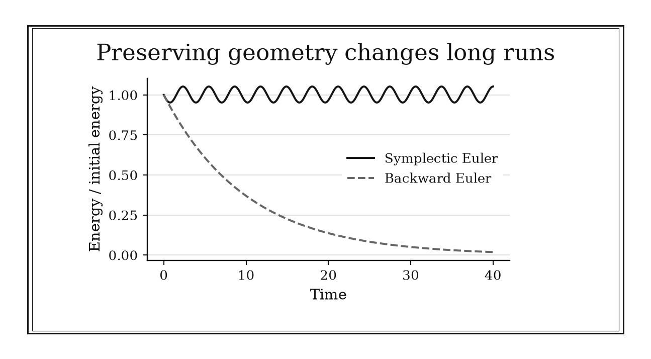
Figure 22.1. For a harmonic oscillator, backward Euler systematically dissipates energy. Symplectic Euler keeps energy oscillating near its initial value in this stable-step example, without conserving it exactly.
22.1.4: Remember that local ODE error is one power higher than global error
History
A single step’s error estimate and the drift accumulated by the end of a long calculation are not the same number, and treating them as interchangeable overstates a solver’s real payoff. Working at Marshall Space Flight Center in Huntsville, Alabama, Erwin Fehlberg published a 1969 NASA report pairing low-order Runge-Kutta formulas that shared evaluations while producing an error estimate each step. Applied to heat-transfer problems, that estimate let Fehlberg adjust step size instead of a fixed grid, turning local versus accumulated error into something actionable.
The equation
For a stable order-(p) method over fixed time (T),
Here (_{n+1}) is the one-step defect and (e_N) the global error after (N) steps.
How to read it
Each step of a method makes a small mistake, a local error or defect: the gap between what one step computes and the exact solution. A method of order has a defect shrinking like as the step shrinks, one power faster than its global error after many steps, which shrinks only like . The reason is arithmetic: halving doubles how many defects fit in a fixed span, eating back one power of each step’s own gain.
The rule assumes the method stays stable; it leaves open an interval that keeps stretching as the step shrinks, where count and size no longer scale together.
How to use it
Forward Euler, a first-order method (), is projecting long-duration liabilities for an actuary checking accuracy against a finer reference. At an annual step the endpoint misses by , or percent; at it misses by . The ratio matches order one: halving the step halves the error. Assuming quartering instead, the actual result is still , far from the quartering predicts. The actuary escalates to a higher-order method rather than shrinking Euler’s step further.
If a policyholder-behavior term amplifies perturbations sharply, error can grow faster than predicted, and the ratio test misses it. This is an Independent rule: once method order, stability, and fixed-time assumptions are known, it directly translates local accuracy into global accuracy scale.
22.1.5: Resolve oscillations with several steps per shortest period
History
A published integration scheme can carry an implicit lesson about resolving repeated motion without stating a target number of points per cycle. Ronald Ruth’s 1983 canonical integrator, built at Brookhaven National Laboratory in New York, was designed for accelerator orbits repeating an enormous number of times, where a small phase error on each pass could accumulate into a real position error. Ruth’s paper never prescribed a fixed count of steps per period. What survived: stability at a frequency is separate from tracking its phase over many cycles.
The equation
If (_{max}) is the highest important angular frequency, then
is a useful starting range.
How to read it
Every repeating motion has a shortest important period . A method approximates that rotation with a built-in amplification factor, and even when its size is fine, meaning stable, its angle, the phase, can still be slightly wrong. A small phase error barely shows after one cycle, but over thousands of cycles it shifts where peaks and resonances land.
Roughly ten to twenty steps across the shortest period, with to , keeps phase slip trustworthy for a while. The count is a starting budget, not a theorem: tens of thousands of cycles can need a stricter number than a few.
How to use it
A kHz switching transient on a series-compensated line is being simulated by a power-grid protection engineer tuning a relay’s trip timing. The period is s, so the rule gives between s and s. The engineer integrates at s, halves it to s, and compares trip time and phase across a second stretch, the horizon the settings must survive.
If the runs agree, the coarser step is trusted for production; if trip timing shifts, the engineer tightens further. The budget assumes kHz is the highest important frequency: an unmodeled harmonic needs its own period folded into , a gap refining the wrong frequency would never reveal. This is an Independent rule: it gives a portable first step size from the shortest scientifically relevant period.
22.2: Control Error Without Missing Events
Adaptive integration succeeds only when the normalized error represents every state component and the controller responds to the correct error order. Events require a separate localization problem; a dense output grid is neither efficient nor a guarantee that a crossing was found.
22.2.1: Scale ODE error with atol plus rtol times state magnitude
History
Get a solver’s error tolerances wrong and a trace species near zero and a bulk quantity far from it get judged by a yardstick built for the other. In 1983, at Lawrence Livermore National Laboratory in California, Alan Hindmarsh and collaborators assembled ODEPACK around the LSODE family, exposing componentwise error weights built from both absolute and relative tolerances rather than one shared scale. That design let a solver’s accept-or-reject decision respect a modeler’s own sense of which components mattered.
The equation
A common normalized error test is
Each (_i) has the units of state component (i); () is dimensionless.
How to read it
Relative tolerance, rtol, sets a relative scale for the solver’s local error test away from zero; does not by itself guarantee six correct digits in the final trajectory. Absolute tolerance, atol, is a fixed floor, in that variable’s own units, below which further precision means nothing, and it matters most where a variable sits near zero. Adding them, , and dividing each component’s error by that sum converts every component into one dimensionless ratio the solver combines into an accept-or-reject number.
The rule says how to combine tolerances. The RMS test can pass even when one normalized component error exceeds one, so critical components may need separate checks. Tolerances come from what the modeler needs to trust, and global trajectory accuracy still requires verification.
How to use it
A kinetic model tracking a trace metabolite near mol/L alongside tank temperature near K is run by a brewery’s fermentation technician using a single . Applied alone, that would demand the metabolite be resolved to mol/L, meaningless, while asking temperature to hold only to K, plenty. Instead, the technician sets a metabolite mol/L, near the smallest concentration the tank’s sensors distinguish, and a temperature K, matched to what the recipe needs.
With those floors, the solver stops burning steps on meaningless metabolite digits while still tracking temperature drift that could stall fermentation. A floor too loose, say mol/L, would hide a real depletion event; too tight would make the trace species dominate the run’s cost. This is a Workflow rule: it turns physical error priorities into the solver’s acceptance metric.
22.2.2: Change adaptive ODE steps with the error-order power
History
A fixed step size is either too cautious, wasting effort where the solution barely changes, or too coarse, blowing past accuracy where it moves fast. Erwin Fehlberg’s 1969 NASA report, produced at the same Huntsville rocket center, combined matched low- and higher-order Runge-Kutta formulas so one step yielded both an accepted value and an error estimate. Fehlberg then applied that estimate to heat-transfer problems, letting each step’s size respond to the solution instead of following one fixed grid.
The equation
If the normalized local error behaves as
then a proportional update is
where (0<s<1) is a safety factor and practical implementations cap growth and shrinkage.
How to read it
An adaptive solver estimates its own local error after each step, assuming it behaves like the step size raised to a power, , where is the order. Solving that backward for the step making equal to one gives : a large error shrinks the next step, a small error grows it. Some conventions make the exponent instead, so the estimator’s order must be checked, not assumed.
The safety factor , below one, and caps on growth or shrinkage protect against an estimate that is a poor guide for one step, though the rule cannot locate the moment the power law breaks, such as right after a discontinuity.
How to use it
A clinical pharmacologist is building a dosing-simulation tool around an adaptive fourth-order solver () to trace plasma concentration after a rapid intravenous bolus. Near the injection, the local error estimate returns . Solving the update rule gives : before safety, the next step should shrink by half. With , the factor is , and the solver retries at percent rather than the plain percent the bare power law suggested.
The pharmacologist still checks a cap on step growth or shrinkage, since a wild near the spike can send the step oscillating. If the model switches compartment equations at the bolus moment, the power law briefly stops applying. This is a Specialized rule: it is an internal controller step whose exponent must match the active error estimator.
22.2.3: Locate ODE events with root finding, not output sampling
History
Reporting only the two output times bracketing a crossing, and calling that the event time, throws away information the solver already holds. The ODEPACK family, assembled at the Livermore lab in 1983 by Alan Hindmarsh and collaborators, included LSODAR, adding rootfinding for event functions atop automatic stiff and nonstiff integration. Instead of hoping an output time landed on a crossing, LSODAR searched the interpolant within an accepted step, treating the event’s moment as distinct from print times.
The equation
Define an event surface by
After a crossing is bracketed between accepted endpoints, find
using dense interpolation for (y(t)) and a safeguarded scalar root solve.
How to read it
An event function is a quantity that should equal zero the moment something happens: height above ground, a concentration threshold, a switch condition. An integrator already builds a smooth interpolant spanning each accepted step’s interior, beyond its two endpoints. If is positive at one endpoint and negative at the other, that is a bracket: a root search on the interpolant pins down the crossing far more precisely than the endpoints.
The method finds an ordinary sign-changing crossing reliably. It does not handle an event only touching zero, or a discontinuous breaking the interpolant.
How to use it
A javelin’s flight is being modeled to estimate the landing time, height above ground, by a track-and-field biomechanist. The output grid shows m at s and m at s, bracketing the landing, . Rather than reporting the landing as somewhere between and seconds, a linear bracket estimate, s, is refined using the trajectory model. For a no-drag ballistic segment with acceleration , these endpoint heights imply s. The biomechanist checks this numerical estimate against a force-plate reading and the trajectory’s error budget.
Because vertical velocity changes discontinuously at impact, the biomechanist restarts at with the post-impact velocity rather than integrating through the impact as smooth motion. A tangential bounce grazing zero would not register as a sign change. This is a Workflow rule: it inserts a bracketed localization stage between integration and event-driven state changes.
22.3: Verify Stability, Convergence, and Structure
A successful return code says that one internal contract was met. Credibility needs independent tests: a stability-region check, an observed convergence rate, a conserved quantity, and a linear-algebra design that respects the actual Jacobian structure.
22.3.1: Check explicit Euler against the stability disk
History
A method’s formal accuracy, how small its per-step error is on paper, is no guarantee it is usable at all: accuracy and stability are different questions. From the mid-1950s into the early 1960s, working in Stockholm, Sweden, Germund Dahlquist analyzed multistep methods through a scalar test equation and the region where a method’s numbers stay bounded. A method could be accurate per step and still unusable once its amplification factor landed outside that region. Euler’s disk condition is the plainest case of the two diverging.
The equation
For (y’=y), explicit Euler gives
Absolute stability requires
For real (<0), this becomes (0h/||).
How to read it
For a mode decaying like , explicit Euler multiplies the previous value by , in place of the true decay factor . Stability means that multiplier stays at most one in size, ; the allowed values of form a disk of radius one centered at . For real, negative , that becomes .
Stepping outside that disk does more than blur accuracy: a decaying quantity can start growing or flipping sign each step. The condition screens only this blow-up, saying nothing about accuracy inside.
How to use it
A dairy plant’s pasteurization technician is modeling how fast a contaminant signal decays after heat treatment, , before setting a logging interval. At , the factor is , stable but crude next to the true . At , the factor is : stable, but alternating sign each step. At , the factor is , outside the disk, and the signal doubles every step though the contaminant is dying away.
The technician checks the disk against the fastest decay rate, not the average. A mildly oscillating coupling between pools could hide growth a plain eigenvalue scan misses. This is a Workflow rule: it is a preflight stability check inside an integration decision.
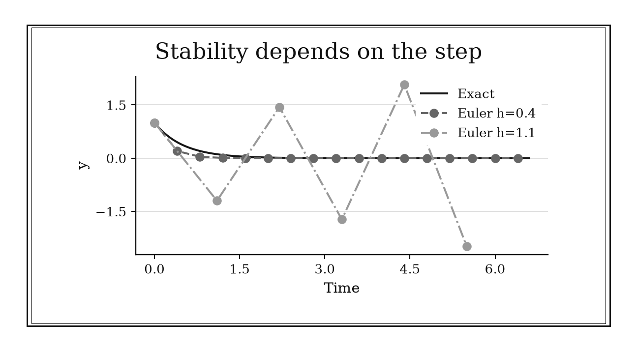
Figure 22.2. For y′=-2y and y(0)=1, explicit Euler has multiplier 1-2h. At h=0.4 it decays; at h=1.1 its magnitude grows with alternating signs, despite the exact solution decaying.
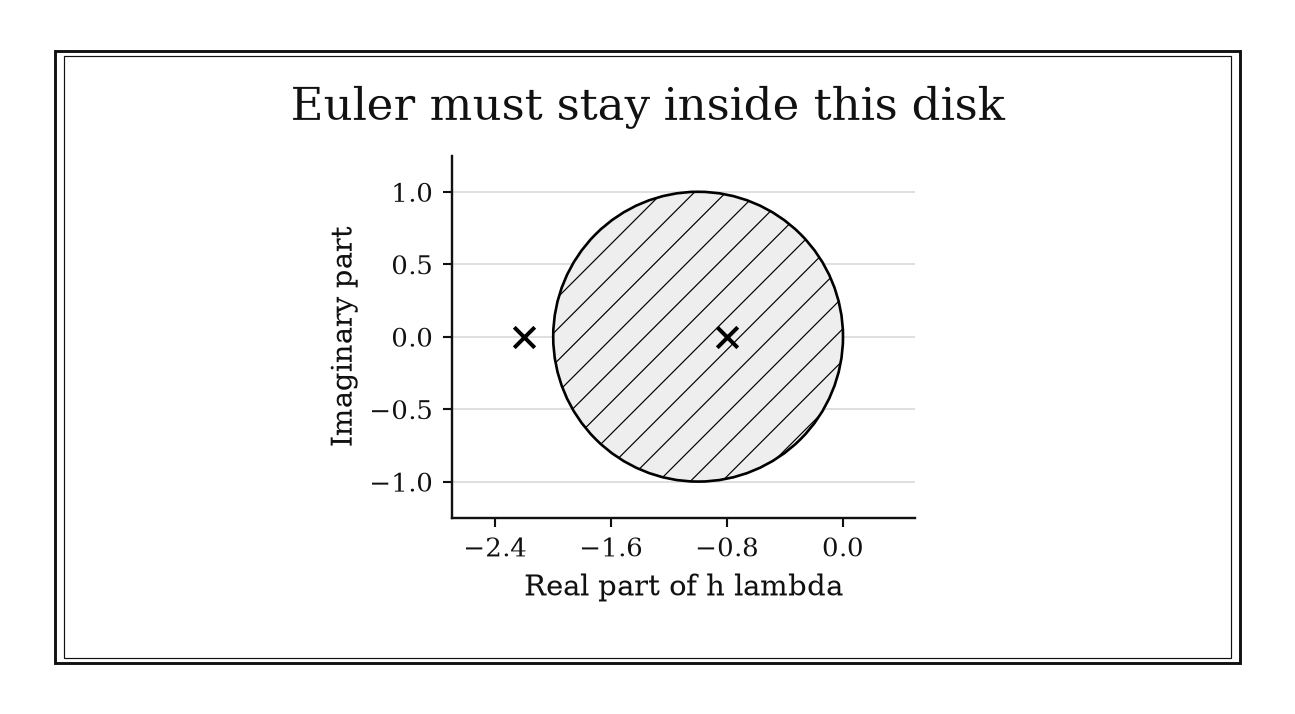
Figure 22.3. Explicit Euler is stable for the scalar test equation when |1+h lambda|<=1. The disk is centered at -1 with radius one; a stable continuous-time eigenvalue alone does not certify a chosen step.
22.3.2: Expect RK4 global error to fall by sixteen on step halving
History
Run a fixed method at successively halved steps, and its output should reveal whether it behaves the way its order promises, without needing the exact answer. Fehlberg’s 1969 NASA work on paired Runge-Kutta formulas made comparing resolutions an everyday habit, since an embedded estimate already required running compatible formulas side by side. That logic supports a check on a fixed method: advance at , , and , and see whether differences shrink at the predicted rate. For classical RK4, the expected global order is four.
The equation
In the asymptotic regime,
so
Without an exact solution, compare successive differences (Y_h-Y_{h/2}) and (Y_{h/2}-Y_{h/4}).
How to read it
Halving the step in a fourth-order method should shrink its leading error term by . Once that term dominates, both the true error and adjacent-run differences shrink by close to that factor. Too coarse a step and higher-order terms muddy the picture; too fine a step and rounding noise flattens the decrease before sixteen.
Comparing three resolutions, not two, guards against a lucky pair. A factor near sixteen supports the code and smoothness together, but does not prove the approached value is correct.
How to use it
An RK4 implementation of a cable’s dynamic-load response is being verified by a bridge engineer before a vibration study. Running the load case at , , and gives endpoint deflection ratios , , and . The differences are and , ratio , matching the fourth-order factor, so the finer step is adopted for the study.
The test confirms only that the method converges at its designed rate, not that the deflection value is correct; a wiring error common to all three runs would pass undetected. An impact event partway through can drop the rate well short of sixteen for reasons unrelated to coding. This is a Workflow rule: it verifies an implementation and chosen resolution against a predicted order.
22.3.3: Monitor invariants as an independent ODE error check
History
A conserved quantity that should never move, mass, energy, total population, gives a trajectory somewhere to fail even when the solver reports every step a success. That is what Ronald Ruth’s 1983 canonical integrator offered almost as a byproduct: designed around Hamiltonian structure rather than a generic error score, it made conserved quantities a natural long-time diagnostic. Watching whether an invariant held tested the calculation against something the accept-or-reject machinery never consulted. The idea travels past the mechanics Ruth solved, to mass, charge, and any quantity a model claims stays fixed.
The equation
For an invariant (I(y(t))=I(y(0))), monitor
where (I_{scale}) prevents meaningless relative error when the invariant is near zero.
How to read it
An invariant is a quantity a differential equation guarantees will not change, arising from an exact cancellation in the equations, not from anything the method adds. Tracking , the relative drift from the starting value, tests whether a solver’s steps preserve that cancellation. Since most solvers do not use to accept a step, a nonzero drift is evidence the accept-or-reject test never saw.
A small, stable drift is reassuring but incomplete: different wrong trajectories can share one conserved total.
How to use it
A public health epidemiologist is running a compartmental disease model, susceptible, infected, recovered, where the population fraction should stay exactly . Checking late in the run, the epidemiologist finds , a drift of , or percent. That number is invisible on any of the three individual curves, each still looking plausible, but it reveals a population-accounting or numerical-implementation problem that the curves do not show. A Runge–Kutta update preserves this linear invariant in exact arithmetic when every stage’s rates sum to zero, regardless of local truncation error.
The epidemiologist checks that every stage’s compartment rates sum to zero, then inspects any clipping, interpolation, implicit-solve residual, and accumulated rounding. Tolerance and step refinement help identify the source, but their response alone does not prove which mechanism caused the leak. This is a Workflow rule: it adds an independent structural test to trajectory verification.
22.3.4: Provide Jacobian sparsity to stiff ODE solvers
History
Treating a large stiff system’s Jacobian as fully dense can turn a minutes-long calculation into one that never finishes, once the state count climbs into the tens of thousands. Alan Hindmarsh’s team at the Livermore laboratory met that wall directly when building LSODES into the 1983 ODEPACK collection, giving the stiff solver a way to exploit sparse Jacobians instead of dense ones. Once a stiff method turns implicit, solving its linearized system each step can dominate every other cost. ODEPACK linked model structure directly to solver performance instead of an always-dense Jacobian.
The equation
For (y’=f(t,y)), define
Large local systems are sparse when
where (n) is state dimension and () counts nonzero entries.
How to read it
The Jacobian collects how strongly each variable’s rate of change responds to every other variable. An implicit step repeatedly solves a matrix built from the Jacobian; a dense version costs roughly numbers to store and operations to solve. Most large models have local coupling, each variable depending on a handful of neighbors, so the nonzero count, , is far smaller than ; supplying that pattern lets the solver skip the zeros. Sparsity changes only cost, never the mathematics, and will not flag an omitted dependency.
How to use it
A geothermal plant engineer is modeling heat diffusion through a rock column with grid points, each coupled only to its two neighbors, a three-point stencil. A dense Jacobian needs stored entries, a factorization no overnight run finishes, while the true count is . Supplying that pattern turns an infeasible -entry factorization into one a laptop can factor every step.
The engineer confirms the pattern includes every coupling that can appear, since an omitted dependency, say a well-injection term coupling distant cells, would be silently missed rather than flagged. A later switching control needs the safe union of every configuration produced. This is a Workflow rule: it carries structural information from the model into the implicit solver’s linear-algebra stage.
Chapter Synthesis: Separate Method Choice From Evidence
ODE reliability begins before the first step. Stiffness asks whether stability rather than accuracy is restricting an explicit method. Dissipative stiffness favors BDF-like formulas; long Hamiltonian motion favors symplectic structure. Formal order explains local and global powers, while points per period protect phase information that stability alone does not preserve.
Adaptive behavior then needs a physical error scale. Absolute and relative tolerances serve different regimes of each state component, and the timestep controller must use the error estimator’s actual order. Events are roots of continuous event functions, not coincidences on an output grid.
Finally, verify with information outside the acceptance test. Place explicit modes inside the stability region. Recover the predicted convergence rate under refinement. Monitor invariants and balance laws. Expose Jacobian sparsity so an appropriate stiff method can perform at the scale the model requires.
Across all twelve rules, ask:
- What numerical obstacle, stability, phase, structure, or event localization, sets the method class?
- Do the tolerances encode the units and importance of every component?
- What independent refinement or invariant check could falsify the computed trajectory?
- Does the rule answer directly, organize the integration workflow, or modify a specialized internal step?
One-Page ODE Toolkit
| Recognition cue | Rule to try | What it gives | Role |
|---|---|---|---|
| Tiny explicit steps after fast transients decay | Diagnose stiffness and compare an implicit solver | Method-class decision | Workflow |
| Large dissipative stiff system | Use variable-order BDF with good Jacobians | Efficient stiff integration | Workflow |
| Long smooth Hamiltonian trajectory | Use a stable, sufficiently small symplectic step and check phase | Conditional long-time energy control | Workflow |
| Confusion about solver order | Separate (O(h^{p+1})) local from (O(h^p)) global error | Error scale | Independent |
| Highest important oscillation known | Start with 10–20 steps per period | Resolution estimate | Independent |
| States cross zero or use different units | Scale by atol plus rtol times magnitude | Dimensionless acceptance test | Workflow |
| Adaptive steps oscillate or reject | Use the estimator’s error-order power | Controller update | Specialized |
| Threshold or impact occurs between outputs | Root-find a continuous event function | Localized event time | Workflow |
| Explicit Euler applied to decay | Check ( | 1+h | ) |
| RK4 implementation needs verification | Halve (h) and seek a factor of 16 | Observed-order test | Workflow |
| Model has a conserved quantity | Monitor normalized invariant drift | Independent diagnostic | Workflow |
| Stiff Jacobian has local coupling | Supply sparsity or Jacobian products | Feasible linear algebra | Workflow |
Decision Path
- Are accepted explicit steps far smaller than output accuracy seems to require? Inspect Jacobian scales and solver statistics; test a stiff method at the same tolerances.
- Is the system strongly dissipative and large? Try BDF with sparse Jacobians. If it is Hamiltonian and long-time geometry matters, choose a symplectic method instead.
- Does the solution oscillate? Set a starting maximum step from the shortest important period, then verify phase and amplitude under refinement.
- Are state scales heterogeneous or near zero? Choose componentwise absolute tolerances and a dimensionless relative tolerance before judging cost.
- Does the model switch, impact, or cross a threshold? Define a smooth event function and localize a bracketed root; do not shrink the display grid as a substitute.
- Is the method explicit? Check its full stability region against relevant modes, not only its formal order.
- Can the exact solution be avoided? Use three-level refinement, invariant drift, and balance checks as independent evidence.
- Do implicit solves dominate? Expose sparsity and escalate to appropriate sparse or matrix-free linear solvers.
Transfer Problems
1. Diagnose a stiff decay
Consider
integrated from (0) to (10) s. Explain why the visible long-time solution can be smooth while explicit stability demands tiny steps. Choose an integrator family, identify useful solver statistics, and state a refinement check.
2. Build a tolerance and event contract
A model contains temperature near (300) K and a trace concentration near (10^{-9} ). It terminates when temperature first exceeds (350) K. Propose dimensionally meaningful absolute tolerances, one relative tolerance, an event function and direction, and a reason output sampling alone is inadequate.
3. Verify an oscillatory trajectory
A Hamiltonian oscillator has shortest relevant period (0.02) s and a known energy invariant. Choose a starting fixed step, describe a symplectic integration option, predict how RK4 endpoint error should change under step halving, and specify what energy behavior would trigger escalation.
Where These Ideas Reappear
- Partial differential equations: method-of-lines discretizations inherit stiffness, CFL limits, sparse Jacobians, and coupled time–space error budgets.
- Control theory: closed-loop poles, sampling intervals, delay, and events create the same stability-versus-resolution distinction.
- Signal processing: points per period becomes sampling and frequency-resolution planning; phase error becomes spectral or filter distortion.
- Optimization: implicit ODE steps are nonlinear solves whose scaling, sparsity, and stopping criteria determine practical cost.
- Scientific computing: profiling, sparse data structures, and reproducible refinement studies turn a solver run into auditable evidence.
- Mechanics and molecular simulation: invariants and symplectic geometry matter more than a single short-time local error number.
Historical Notes and Sources
All twelve profiles use verified historical stories. The chapter separates each documented contribution from the modern operational wording and numerical thresholds.
- Petzold and automatic stiffness switching: original SIAM paper; SIAM article record.
- Curtiss, Hirschfelder, and BDF: original 1952 PNAS paper; PNAS full-text record.
- Ruth and symplectic integration: original IEEE paper; CERN record and full text.
- Fehlberg and embedded Runge–Kutta control: NASA Technical Report R-315; Google Books record.
- ODEPACK tolerances, events, and sparse Jacobians: LLNL ODEPACK record; Netlib source archive.
- Dahlquist and stability regions: Dahlquist’s BIT paper; historical review.
- Modern numerical statements and implementation
guidance: SciPy
solve_ivpreference; Driscoll and Braun, Fundamentals of Numerical Computation; PETSc linear-solvers manual.