Chapter 23: Partial Differential Equations: Discretize, Resolve, and Verify
Halving a mesh spacing sounds like a twofold refinement. For an explicit heat calculation, it can force roughly four times as many time steps, while a multidimensional grid also multiplies the number of cells to update. A harmless-looking resolution decision can therefore change both stability and total cost by orders of magnitude.
Partial differential equations add spatial choices to every temporal choice. A stencil must respect the direction of information flow. A conservative law should balance shared fluxes. Waves, shocks, and boundary layers need different notions of resolution. Even a stable, smooth contour plot may be converging to the wrong boundary-value problem or hiding a coding error.
The fifteen rules in this chapter form three themes. The first chooses spatial discretizations that respect transport, conservation, discontinuities, and regularity. The second budgets timestep and mesh resolution against physical scales. The third demands stability analysis, manufactured verification, observed convergence, boundary independence, and scalable elliptic solves.
The governing habit is: make the discrete information path match the PDE, then try to falsify the computation with refinement and independent tests.
23.1 , Choose a Spatial Discretization That Respects the Physics
A spatial formula carries physical commitments. Upwind bias follows characteristics; finite-volume fluxes enforce local balance; nonlinear limiting sacrifices formal order at a discontinuity to prevent invented extrema. Choose those commitments deliberately.
23.1.1: Bias transport discretization upwind
History
Which side of a moving front should a formula trust: the direction a value arrives from, or an average of both neighbors? In August 1952, Richard Courant, Eugene Isaacson, and Mina Rees answered that for nonlinear hyperbolic equations, equations that transport a quantity rather than smooth it out, working in New York. Their stencil read each cell from the side the flow arrived from, the characteristic direction information travels along: the documented ancestor of upwind discretization. Respecting that direction earns the scheme its stability.
The equation
For (u_t+a u_x=0), use
and
The selected neighbor lies on the incoming characteristic side.
How to read it
Rightward flow reads the slope from the current cell and the one to its left, the direction values arrive from; leftward flow reads from the right. The cost is numerical smoothing: a sharp step blurs across more cells as it advances, like ink spreading along a wet towel. A centered formula splits the difference between both neighbors instead and can go unstable with a plain forward-time step. The rule does not say how much blurring a given use can tolerate before a front becomes useless.
How to use it
A river-quality engineer models a diesel spill advecting downstream at (a=1.6 ), cells (x=2 ), step (t=1 ): Courant number (1.6/2=0.8). Upwind keeps modeled concentration between background and the spill’s peak, smearing over more cells but staying physical. A centered, forward-time run instead reports concentration below background just ahead of the plume and a spike above the true peak behind it, so the engineer would overstate the spill to a regulator. Because upwind spreads the edge and can shift threshold-crossing times, the engineer pairs it with a limited high-order scheme where the sharp edge matters for an evacuation call. This is a Workflow rule: it chooses the spatial information direction inside a transport discretization.
23.1.2: Use cell Peclet number to judge centered convection-diffusion
History
A centered finite-volume stencil for convection and diffusion, transport that carries a quantity along while spreading it out, can return coefficients with no physical meaning once flow dominates spreading. In 1980, in Minneapolis, Minnesota, Suhas Patankar’s textbook Numerical Heat Transfer and Fluid Flow organized such stencils around the cell Peclet number, a ratio of transport to spreading across one cell, and introduced a hybrid rule abandoning centered differencing once that ratio grew too large. The threshold below belongs to that one stencil, not every mesh.
The equation
For steady one-dimensional transport with speed (a), diffusivity (D), and cell width (x), define
A centered stencil remains monotone in the basic uniform-grid model when approximately
How to read it
The numerator measures how much a quantity is carried past a cell by flow; the denominator measures diffusion, spreading and smoothing, through the same cell. Past a ratio of about two, a centered stencil’s neighbor coefficients flip sign, rippling above and below the real answer near a steep gradient, the way a too-stiff spring overshoots instead of settling. This is a cell-by-cell condition: a modest reactor-wide average does not guarantee safety in locally coarse cells or regions with faster flow or weaker diffusion. It flags when centered differencing is untrustworthy, not how large the ripple will be.
How to use it
A plant operator models reactant concentration with (a=1 ), (D=10{-3} 2/). Safe spacing needs (x2D/|a|=0.002 ). The plant’s mesh uses (x=0.01 ), giving (|Pe_h|=0.01/10^{-3}=10), five times the threshold, so the smooth-looking output likely hides unphysical oscillations near a steep boundary layer. Refining to (0.002 ), or switching to upwind, removes the ripple. Before either fix, the operator reruns at two mesh sizes and checks the profile stays bounded between feed value and zero. This is a Workflow rule: it is a discretization guardrail that converts local convection–diffusion competition into a method or mesh decision.
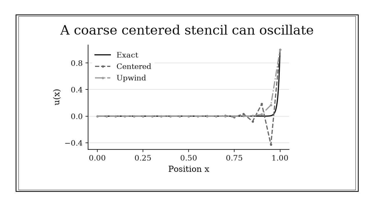
Figure 23.1. For steady a u′-D u″=0 with a=1, D=0.01 and mesh width 0.05, cell Peclet number is five. Centered differencing oscillates; upwind stays bounded but smears the boundary layer.
23.1.3: Prefer finite volume when local conservation is nonnegotiable
History
A staggered grid of pressure and velocity, tracked cell by cell with marker particles riding a free surface: that is the artifact Francis Harlow and Eddie Welch published in December 1965 in Los Alamos, New Mexico, for time-dependent incompressible flow. Their method balanced flow crossing each cell’s faces so exactly that conservation became algebraic, not a hope pinned on a carefully taken derivative. Marker-and-Cell is historically a finite-difference formulation, but its face-by-face balancing already contains the finite-volume idea used here: one flux per interior boundary, shared by both cells it touches.
The equation
For cell average (q_i), numerical face flux (F), and source average (s_i),
The same interior face flux is used by both adjoining cells with opposite signs.
How to read it
A cell average (q_i) is a quantity’s typical value inside one chunk of the domain, and a face flux (F) is how much crosses one cell wall per unit time. The same computed flux is subtracted from one cell and added to its neighbor, so summing every cell’s update cancels every interior face, leaving only what crosses the outer boundary, where a boundary condition, a rule fixing value or flux there, applies. That survives a discontinuity, an abrupt jump, since it needs only integrated balance. It does not guarantee accuracy or positivity.
How to use it
Oxygen moving through a three-segment ventilator circuit gives a biomedical engineer face fluxes to check: (F_{1/2}=0.42), (F_{3/2}=0.42), (F_{5/2}=0.31), (F_{7/2}=0.31) liters per minute. Summing the three cells cancels the shared interior fluxes, leaving inlet (0.42) and outlet (0.31): net (0.42-0.31=0.11). If the software reports the tubing gaining or losing oxygen beyond that (0.11), the code has a defect or inconsistent junction coupling. The balance can close exactly at (0.11) while one segment’s own concentration is still wrong, since conservation checks the sum, not each term. The engineer audits that every junction shares one computed flux and a consistent sign convention. This is a Workflow rule: it selects an integral discretization whose algebra matches a conservation law.
23.1.4: Limit high-order reconstructions near discontinuities
History
Get monotonicity wrong at a shock and a simulated flow can show a density spike or dip that never existed, undermining every prediction downstream. Working in Leiden in March 1974, Bram van Leer published the second paper in his “ultimate conservative difference scheme” series, seeking a transport method that kept second-order accuracy without inventing false extremes. His fix let the reconstructed slope depend on the solution: smooth where data are smooth, flattened toward first order wherever neighboring differences disagree, since a fixed high-order formula cannot stay free of oscillation at every discontinuity, an abrupt jump in the solution.
The equation
One generalized minmod slope is
where (1) and minmod returns the smallest magnitude when all arguments share a sign, otherwise zero.
How to read it
Where the tracked quantity changes smoothly, the difference to the left neighbor roughly agrees with the difference to the right, and the limiter lets a full higher-order slope through. Across a jump or peak the two disagree, so the limiter shrinks the slope, often to zero, and the scheme drops to a plain first-order update right there, giving up accuracy exactly where a high-order formula would overshoot past the true minimum or maximum. It cannot tell a genuine sharp feature from noise shaped the same way.
How to use it
A congestion shockwave behind a lane closure gives a traffic engineer three segment densities to model: (q_{i-1}=0), (q_i=0), (q_{i+1}=1). Backward difference (0) and forward difference (1) disagree, so minmod returns a slope of zero at segment (i), keeping the reconstruction flat rather than extrapolating between very different neighbors. That zero keeps density between 0 and 1; an unlimited reconstruction could send it below 0 or above 1, meaningless for a road. The same limiter can flatten a smooth density rise near a merge that is not a jam, understating how fast congestion is building. The engineer trusts the occupancy output for ramp-metering timing but flags merge-zone readings for the limiter’s clipped peak. This is a Specialized rule: it modifies the reconstruction stage of a shock-capturing method.
23.1.5: Do not expect finite-element order beyond solution regularity
History
Doubling a finite-element mesh’s polynomial degree can fail to buy the extra convergence the formula promises, for reasons that have nothing to do with coding. A 1972 symposium volume from the University of Maryland, edited by A. K. Aziz and held in Baltimore County, Maryland, gathered foundational finite-element theory built by Ivo Babuska, Aziz, and collaborators, making a solution’s available smoothness, its regularity, an explicit ceiling on convergence alongside degree. A higher-degree element supplies more capacity, but that capacity is wasted once the solution runs out of derivatives to exploit.
The equation
For degree-(p) conforming elements and (uH^s), a representative energy-norm estimate is
The precise statement also depends on mesh quality, coefficients, geometry, and the variational problem.
How to read it
Polynomial degree (p) is how rich a shape the method fits inside each element; regularity (s) describes square-integrable weak derivatives, or fractional smoothness when (s) is not an integer; it does not mean (s) continuous derivatives. The estimate uses whichever is smaller: raising (p) keeps paying off only until it passes (s-1). A sharp interior corner, like the reentrant corner of an L-shaped bracket, can hold the solution to barely more smoothness than a first derivative no matter how high a degree the elements use elsewhere. The estimate is a ceiling, not a promise: quadrature error, from approximating an integral, can push the observed rate lower still.
How to use it
A structural engineer uses quadratic displacement elements for an L-shaped steel bracket. With sufficient regularity, the displacement’s energy-norm error can decrease like (h^2), quartering under mesh halving. A reentrant-corner singularity can reduce the available regularity: if the relevant estimate has (s=1.5), its uniform-mesh rate is only (h^{1/2}), a factor of () per halving. This norm estimate does not certify pointwise peak stress, which may be unbounded at an ideal sharp corner. The engineer uses graded meshes and evaluates a defined stress quantity, checking whether a physical corner radius is needed. This is a Workflow rule: it diagnoses when regularity, rather than polynomial degree, controls the refinement strategy.
23.2: Respect Time-Step and Resolution Scales
The mesh and timestep together define what the numerical model can communicate and resolve. Hyperbolic information must not outrun the stencil, diffusion creates a quadratic step restriction, and physical features need far more than the two samples required merely to represent a sinusoid.
23.2.1: Keep explicit advection CFL near or below one
History
Pick too large a time step for an explicit transport code and the calculation can blow up entirely, exponentially amplifying every small error, however fine the mesh. In 1928, in Gottingen, Germany, Richard Courant, Kurt Friedrichs, and Hans Lewy proved that convergence for a hyperbolic problem, transport rather than diffusion, requires the scheme’s domain of dependence, everything one update can see, to contain the true physical domain of dependence, everything the answer depends on. Squeezing the mesh ratio to satisfy that is the origin of the CFL condition; the Courant number near or below one is only its simplest reading.
The equation
For speed (a), timestep (t), and cell width (x),
First-order explicit upwind advection requires
Other integrators, reconstructions, dimensions, and grids have different stability limits.
How to read it
In one step, a disturbance travels a distance equal to speed times step length. The Courant number () compares that distance to one cell’s width: past (), the disturbance has outrun the single neighboring cell the stencil can see, missing information the answer depends on. That mismatch, not a bad coefficient, causes the instability. With several signals at once, use the fastest local speed; the slowest offers no protection. CFL compliance guarantees neither accuracy nor stability for a different spatial discretization.
How to use it
A warehouse ventilation engineer models exhaust gas at (|a|=30 ), mesh (x=0.01 ): limit (t/30=3.33^{-4} ); target Courant (0.8) tightens that to (2.67^{-4} ). Running instead at (t=5^{-4} ) to save overnight compute time gives Courant number (30^{-4}/0.01=1.5), above one, and the field would grow without bound within a few hundred steps rather than settle. The limit must be recomputed whenever velocity or spacing changes, including at a narrowing junction. When one bottleneck section would force the whole simulation to a punishing global step, the engineer escalates to local time stepping there instead. This is a Workflow rule: it converts physical propagation speed and numerical reach into an explicit timestep guardrail.
23.2.2: Remember that explicit diffusion steps scale with mesh size squared
History
A finer mesh can force many more time steps once an explicit heat-conduction scheme is chosen. In 1947, in Cambridge, United Kingdom, John Crank and Phyllis Nicolson compared finite-difference schemes for the heat equation, a parabolic equation, spreading a quantity over time rather than transporting it, and introduced their own time-centered implicit method, solving every cell together rather than one at a time. Their comparison made a fact about the explicit alternative visible: its stable step shrinks with the square of mesh spacing, the quadratic penalty this rule tracks.
The equation
For forward Euler with centered diffusion in one dimension,
On an equal-spacing (d)-dimensional Cartesian grid, a common bound is
How to read it
The mesh’s finest wiggles decay fastest as it gets finer, at a rate proportional to diffusivity over the square of cell spacing. Forward-time stepping stays stable only if the time step keeps pace with that fastest-decaying wiggle, forcing (t) to shrink like (x^2): halving spacing cuts the allowed step by about four, before counting the extra cells needing updates. That quadratic scaling is a stability limit, not the step giving best accuracy for least cost.
How to use it
Heat penetrating a planar steel slab sets a simulation specialist’s mesh, ({-5} 2/), (x=10^{-3} ) through the slab’s thickness: limit (t{-6}/(2{-5})=0.05 ), so an eight-hour furnace soak needs roughly (576{,}000) steps. Halving (x) to (0.5^{-3} ) for the near-wall gradient drops the limit to (0.0125 ), quadrupling step count for that mesh alone. Pushing resolution further could make an explicit run impractically slow for routine validation. Switching to an implicit or IMEX integrator removes this explicit diffusion stability restriction when diffusion is treated implicitly, while spatial work and accuracy requirements remain; each step instead carries a solve, worth it once step count becomes the bottleneck. This is an Independent rule: under the stated stencil assumptions, it directly estimates the explicit diffusion timestep scale.
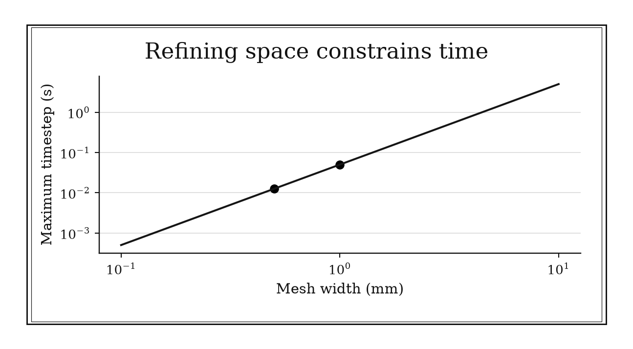
Figure 23.2. For one-dimensional centered diffusion with forward Euler and alpha=10^-5 m²/s, the stability ceiling is dx²/(2alpha). Halving dx from 1 mm to 0.5 mm quarters the ceiling from 0.05 s to 0.0125 s.
23.2.3: Resolve waves with at least about ten cells per wavelength
History
More than two points per shortest cycle are the ideal bandlimited sampling threshold, but that bound has nothing to do with whether a simulated wave keeps its shape over distance. Frank Ihlenburg and Ivo Babuska demonstrated this on 30 November 1995, in College Park, Maryland, analyzing finite elements for the Helmholtz equation, an equation for a single steady wave frequency, and showed that numerical phase error, simulated speed drifting from true speed, grows with wavenumber even at fixed formal order, a defect sometimes called pollution error.
The equation
For the smallest wavelength that must be accurate,
is a starting range for common low-order methods.
How to read it
Sampling strictly above twice the highest frequency can prevent ideal bandlimited aliasing, but says nothing about whether the wave arrives at the right place at the right time after traveling any distance. Every discrete spatial formula has its own numerical dispersion, simulated speed depending on wavelength in a way the true wave does not; phase error stays small only with many points per wavelength, not two. Ten to twenty is a starting range for low-order methods. The rule sets a first mesh size; it does not certify shocks, boundary layers, or anything besides a smooth traveling wave.
How to use it
A consultant reviewing a speaker-cabinet manufacturer’s mesh checks a 2 kHz resonance in air, sound speed 340 m/s: wavelength (/2000=0.17 ). Ten to twenty cells per wavelength calls for cell size between (0.17/20=8.5 ) and (0.17/10=17 ). The team’s mesh, reused from a 500 Hz model, has (30 ) cells, only (0.17/0.03) per wavelength at 2 kHz, and can look smooth on screen while quietly reporting the resonance at the wrong frequency, since dispersion error accumulates over reflections rather than showing as jaggedness. Refining to roughly 10 mm and rerunning at two densities confirms the resonance has stopped shifting. This is an Independent rule: it supplies a portable first spatial scale from the highest important wave frequency.
23.2.4: Place several cells across every boundary layer
History
A short paper at the 1904 International Congress of Mathematicians split fluid flow past a surface into two regions and quietly launched a century of engineering mesh design. Ludwig Prandtl presented it on 12 August 1904 in Heidelberg, Germany: even where viscosity, a fluid’s resistance to shearing, is small almost everywhere, it stays a leading-order effect inside a thin layer at the wall, where velocity changes fast. Outside it, flow looks smooth and nearly inviscid; the decisive shear and drag live inside that layer, and “several cells across it” is a later habit, not Prandtl’s own number.
The equation
If a layer has thickness (), begin with
where (n_{wall}) is wall-normal spacing. Method order and the desired wall output determine the final count.
How to read it
A quantity changing by (u) across a layer of thickness () has a derivative on the order of (u/), steep in proportion to how thin the layer is. A mesh built from cells the size of the whole domain averages that change to nearly nothing. Because the gradient runs across the layer, not along it, refinement can be directional: many thin cells stacked wall-normal, ordinary cells along the wall. The rule says how many cells to place once thickness is known, not the thickness itself, which needs a separate estimate.
How to use it
Airflow over a time-trial cycling helmet sets the boundary-layer thickness a graduate student running the study must resolve ahead of separation, ( ). Ten cells across calls for wall-normal spacing (n_{wall}/10=0.05 ), far finer than the (5 ) cells used over the rest of the body. Reusing that coarse spacing near separation, where drag is decided, would place well under one cell across the layer, making the drag estimate unreliable for deciding whether the design saves a rider meaningful time. Grading the mesh from (5 ) to (0.05 ), then refining once more and comparing drag and wall shear, tests whether those outputs have converged. This is a Workflow rule: it converts a localized physical scale into a directed mesh-design requirement.
23.2.5: Balance temporal and spatial discretization errors
History
A costly calculation can buy nothing when it refines the wrong axis: pouring effort into a finer mesh while the timestep already dominates the error changes the answer by less than roundoff. Lewis Fry Richardson confronted a related problem in 1911, working across several mesh spacings in the United Kingdom to compute stresses in a masonry dam. He compared results across that sequence and read the pattern of change as evidence of how fast the true error was shrinking. Balancing spatial error against timestep error extends that same measured pattern.
The equation
In an asymptotic regime, model the leading numerical error as
An economical target is
unless stability forces a smaller timestep.
How to read it
Model the leading error as two terms added together: one shrinking with mesh spacing to power (p), the other with timestep to power (q). If one term is already far smaller, refining it further barely moves the total, like tightening one loose bolt when the other three legs still wobble. An economical target makes both terms comparable, so each refinement buys proportional improvement. This holds only where the leading terms describe the error; if the two sources partly cancel, the total can look deceptively small while one is still large.
How to use it
An option-pricing scheme, second order in both the price mesh and the time step, lets a derivatives quant test where refinement pays off. Fixing a very fine time step, the quant refines the price mesh alone and measures spatial order (p) with constant (C_x); fixing a fine mesh and refining time alone gives (q) with comparable constant (C_t). Since both leading terms start roughly equal, halving only the price mesh, cells (200) with the time step unchanged, changes cost by (), not (), while reducing the leading error sum from to if each initial contribution is , a 37.5% reduction; time error then dominates. Halving both together, cells (200) and timestep also halved, raises cost (2=4)-fold, worth paying for. This is a Workflow rule: it allocates accuracy and cost across two discretization stages.
23.3: Prove That the Computation Solves the Intended PDE
Verification asks whether the equations were discretized and implemented correctly. It precedes comparison with experiments. Amplification factors test a linear scheme, manufactured fields expose code defects, refinement measures order, boundary movement tests domain truncation, and multigrid makes repeated elliptic verification affordable.
23.3.1: Require every Fourier amplification factor to stay bounded
History
A finite-difference scheme can look reasonable on paper and still blow up the moment it runs, growing without bound for no visible reason. John Crank and Phyllis Nicolson’s 1947 stability analysis of their heat-equation scheme became a standard setting for catching that failure early: decompose the solution into periodic Fourier modes, waves of every wavelength the grid can represent, and track how one step multiplies each. A fixed-coefficient stencil treats every mode independently, so one multiplier over one grows exponentially, swamping the true solution.
The equation
Insert a discrete Fourier mode
For a non-growing stability target, require
More generally, the bound must match the PDE’s permitted growth over the interval.
How to read it
Insert a periodic wave into the update formula and it returns multiplied by one number, the amplification factor (G), whose size controls growth or decay each step. Requiring the largest (|G|) over every wavenumber to stay at or below one keeps every mode from blowing up, like checking every student’s score rather than just the class average. Passing proves the scheme will not diverge for a linear, constant-coefficient, periodic problem; it says nothing certain about boundaries, changing coefficients, or nonlinear terms, where growth can appear by a route this test cannot see.
How to use it
A medical-physics team verifies an explicit model of tissue heating for a hyperthermia treatment plan, forward-Euler diffusion with (G()=1-4F^2(/2)). The worst mode sits at (=), giving (G=1-4F); requiring (|G|) forces (F/2). The team’s planned setting gives (F=0.6), so (G=1-4=-1.4), outside the bound. Run there, modeled tissue temperature would oscillate and grow rather than settle, an artifact mistakable for a genuine unstable hot spot that could change a clinical planning decision. Halving the time step to (F=0.3) gives (G=-0.2), inside the bound. Passing this test does not confirm accuracy, nor that boundary conditions and the perfusion source term are handled correctly. This is a Workflow rule: it verifies a scheme’s modal stability before production use.
23.3.2: Verify PDE codes with a manufactured solution
History
Unit tests can certify every subroutine of a PDE solver; nothing certifies that the assembled code converges at its claimed rate. Stanly Steinberg and Patrick Roache built a fix in 1985, working in Albuquerque, New Mexico: use symbolic manipulation to pick an arbitrary smooth field, substitute it into the governing equations, and let the algebra generate the forcing and boundary data a correct code should reproduce, reversing the usual order by choosing the answer first.
The equation
For differential operator (L), choose a smooth (u_{exact}) and set
Then solve
with boundary and initial data taken from (u_{exact}), and measure (|u_h-u_{exact}|).
How to read it
Choose a smooth function, run it through the differential operator, and whatever comes out becomes the forcing term the code must reproduce; boundary and initial values are read straight off the same function. Because the exact answer is known by construction, any mismatch is attributable to implementation and discretization, not a shaky physical model. Every term, coordinate transform, coupling, and boundary branch can be exercised by choosing a field complicated enough. A field need not be physically realizable, but one so simple the discrete operator reproduces exactly can hide errors.
How to use it
A graduate researcher verifies a second-order groundwater-flow discretization with (u=(x)(y)) on the unit square for (-u=f), forcing (f=2^2u), zero on all four boundaries. Running three successively refined meshes and measuring (L^2) error, the researcher expects error to fall by close to (4) each halving, the signature of second-order convergence. If error barely changes between the second and third mesh instead, the researcher checks solver tolerance, roundoff, and whether the asymptotic regime has been reached, then investigates a possible implementation defect. Because this field already satisfies zero boundaries, a second field with a nonzero boundary value tests that path before trusting the solver on a real, non-rectangular aquifer. This is a Workflow rule: it creates a controlled exact benchmark for the full discretization pipeline.
23.3.3: Estimate PDE order from normed errors on successive meshes
History
A method’s textbook convergence order is a claim about its formula; whether it shows up in a real calculation only a numerical experiment can settle. Lewis Fry Richardson settled it for one case in 1911: computing stresses in a masonry dam across a sequence of mesh spacings, he read the changing answer itself as evidence of how fast the true value was being approached, extrapolating toward the stress field a still finer mesh would reach. That comparison is the prototype behind every modern grid-convergence study.
The equation
If (E_hCh^p), then two meshes give
Use at least three meshes so two adjacent observed orders can be compared and pre-asymptotic behavior can be detected. A log–log error plot should approach a straight line with slope (p).
How to read it
Refining a mesh by ratio (r) should shrink the leading error by (r) raised to order (p), so measuring errors against a known solution or sufficiently accurate reference and taking a logarithm of their ratio recovers (p). Without such a reference, compare differences on at least three meshes after mapping outputs to a common representation. That number is meaningful only if measured the same way on every mesh, with other sources already pushed below it. A single pair can mislead: pre-asymptotic behavior, where the mesh is not yet fine enough, can look like a clean order when it is not.
How to use it
A bridge engineer verifies a deck-deflection solver on three successively halved meshes, errors (0.020), (0.0051), (0.00128) against a known case. Observed order between the first two is (p_{12}=(0.020/0.0051)/(2)), and between the second and third, (p_{23}), both near the advertised second order, giving confidence in the solver. Stopping after only two meshes and reporting (p_{12}) alone, an artifact of that coarser, still pre-asymptotic pair, could have passed for full verification. The engineer reports refinement ratio, norm, and solver tolerance so a reviewer can reproduce the slope; a welded-joint stress concentration the benchmark lacks makes a locally lower order there expected, not a bug. This is a Workflow rule: it verifies asymptotic convergence through measured, normed refinement evidence.
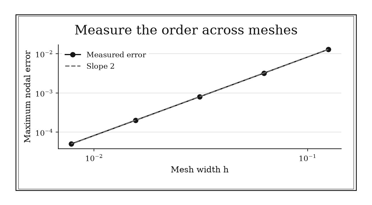
Figure 23.3. For -u″=pi² sin(pi x), u(0)=u(1)=0, centered differences converge to sin(pi x) at approximately second order. Each error is the maximum absolute nodal error on that mesh.
23.3.4: Move artificial boundaries until the answer stops moving
History
A mesh refined inside a truncated domain can converge beautifully to the wrong problem, since cutting an unbounded domain to a finite box is its own approximation, separate from mesh fineness inside. On 13 July 2009, in Washington, D.C., NASA adopted Standard 7009, requiring documented credibility practices, sensitivity, verification, validation, uncertainty, acceptance criteria, for every modeling choice, including where a domain is cut off. The standard hands down no single boundary distance; it documents the duty to test a choice that can move the answer as surely as mesh spacing.
The equation
For reported output (Q(R)) and boundary distance or domain scale (R), require
where (_Q) is tied to the decision’s accuracy requirement.
How to read it
Truncating an infinite domain to a finite box changes the mathematical problem, even if the physical problem is unbounded. A mesh refined finer inside that box will converge smoothly, but to the truncated problem’s answer, not the real, larger domain. Moving the boundary outward and rerunning tests that approximation directly, holding near-field resolution comparable so only domain size changes. One pair of distances agreeing is weak evidence, since boundary and mesh errors can cancel by coincidence; more than one move is needed to see whether output is settling or oscillating from reflection.
How to use it
A rotor-dynamics consultant models the wake behind an offshore wind farm: velocity deficit at the same fixed near-farm observation point is (6.2%), (6.0%), and (5.97%) when the outer boundary is placed at (10D), (20D), and (40D), respectively, with (D) the rotor diameter. With tolerance (0.1) points, the change from (10D) to (20D) is (6.2-6.0=0.2), failing; from (20D) to (40D) it is (6.0-5.97=0.03), passing, supporting agreement of the (20D) and (40D) calculations at the chosen tolerance. The consultant reports the (40D) result and uses another boundary move if stronger evidence is required; this pair alone does not prove the remaining truncation error. Repeating both at comparable near-turbine resolution rules out mesh refinement as the cause. The consultant also checks hub velocity, a near-field quantity, since reflections off an undersized boundary can contaminate local flow while one integrated output stays nearly unchanged. This is a Workflow rule: it verifies domain-truncation independence as a separate credibility dimension.
23.3.5: Use multigrid when elliptic solves dominate
History
A solver visiting each unknown only a small, roughly fixed number of times, however many unknowns the grid has, sounds too efficient for an elliptic problem, a steady equation, like Poisson’s, whose solution at any point depends on the whole domain at once. Achi Brandt published exactly that in April 1977, working in Rehovot, Israel: a multilevel method combining relaxation, a cheap local smoothing sweep, on the finest grid, with a correction from a coarser one, repeated across several levels, reporting work for Poisson-type problems scaling with unknown count, not faster.
The equation
For (N) unknowns, an effective geometric or algebraic multigrid V-cycle aims for
and
with () nearly independent of mesh spacing.
How to read it
Relaxation, a repeated local averaging update, quickly damps jagged error that changes a lot cell to cell, but barely touches smoothly varying error, since neighbors look nearly alike to a local update. Move that smooth error to a coarser grid, where it looks jagged again, cheap to remove there. Cycling down through several levels and back up removes error at every scale for roughly constant work per unknown, the near-linear claim in the rule, depending on the smoother and coarse problem matching the operator well.
How to use it
A municipal water utility solves a large elliptic pressure equation for its network, where each multigrid V-cycle, one down-and-up sweep through the levels, reduces the residual, the remaining imbalance, by a factor of (0.1). Bringing that down six orders of magnitude needs about (6) cycles, since (0.16=10{-6}), whether the model has (10^5) unknowns or (10^8), provided the measured factor remains near 0.1 on both meshes. Work per cycle being linear in unknown count does not by itself guarantee that mesh-independent contraction. Used as a preconditioner rather than a standalone solver, engineers also track an output quantity, since a shrinking residual alone does not guarantee it converged. High-contrast valves added later introduce coefficient jumps plain multigrid handles poorly, degrading convergence below the six-cycle expectation. This is a Workflow rule: it selects a multilevel linear-solver strategy when repeated elliptic work controls the PDE computation.
Chapter Synthesis: Make Credibility Multidimensional
A PDE result must satisfy several independent contracts. Its stencil should follow characteristic direction, preserve required balances, and control reconstruction near discontinuities. Its approximation order cannot exceed the solution regularity available to support it.
Resolution then joins physics to cost. CFL limits how far explicit information can travel per step. Diffusion adds a quadratic mesh penalty. Waves need cells per wavelength, boundary layers need directed cells across their thickness, and space and time errors should share a deliberate budget.
Verification closes the loop. Fourier factors expose unstable modes. Manufactured solutions test the full implementation against an exact field. Successive meshes measure observed order. Moving artificial boundaries isolates domain error. Multigrid keeps elliptic verification affordable at large scale.
Across all fifteen rules, ask:
- Does the discrete information flow and conservation structure match the PDE?
- Which physical feature sets the smallest spatial and temporal scale?
- Have code, mesh, timestep, boundary, and linear-solver errors been varied separately?
- Is the rule a direct estimate, a workflow choice, or a specialized reconstruction step?
One-Page PDE Toolkit
| Recognition cue | Rule to try | What it gives | Role |
|---|---|---|---|
| Directed transport | Bias the stencil upstream | Stable baseline discretization | Workflow |
| Convection competes with diffusion | Check ( | Pe_h | ) against about 2 |
| Local balance is mandatory | Use shared finite-volume face fluxes | Algebraic conservation | Workflow |
| Shocks or contacts are present | Limit high-order reconstruction | Nonoscillatory interface states | Specialized |
| FEM order stalls near singularities | Compare (p) with solution regularity | Refinement diagnosis | Workflow |
| Explicit hyperbolic update | Keep method-specific CFL within limit | Timestep bound | Workflow |
| Explicit diffusion | Budget (t=O(x^2)) | Cost and stability scale | Independent |
| Smooth waves propagate | Start with 10–20 cells per wavelength | Resolution estimate | Independent |
| Thin wall or interface layer | Place 8–15 directed cells across it | Mesh requirement | Workflow |
| Space and time refinement plateau | Estimate and balance both leading errors | Error budget | Workflow |
| Linear constant-coefficient stencil | Inspect all amplification factors | Modal stability test | Workflow |
| PDE code lacks an exact benchmark | Manufacture a solution and forcing | Verification case | Workflow |
| Formal order needs evidence | Use normed errors on three meshes | Observed order | Workflow |
| Exterior domain was truncated | Move the boundary and compare outputs | Domain-independence test | Workflow |
| Elliptic solves dominate runtime | Use multigrid or multigrid preconditioning | Near-linear solver path | Workflow |
Decision Path
- Is the PDE transport-dominated? Follow characteristic direction, inspect cell Peclet numbers, and use limiting near discontinuities.
- Must a quantity balance cell by cell? Form one shared numerical flux per face and audit the telescoping global balance.
- Is nominal high order missing? Check solution regularity, geometry, quadrature, and solver tolerance before increasing polynomial degree.
- Is time integration explicit? Evaluate every applicable advection, diffusion, reaction, and source stability restriction.
- Are waves or thin layers important? Set the mesh from wavelength and layer thickness, then refine the output that depends on their derivatives or phase.
- Do space and time errors interact? Isolate each with separate studies before choosing a coupled refinement path.
- Has the code been verified? Run manufactured solutions and recover predicted order in relevant norms.
- Could the domain or linear solve contaminate the answer? Move artificial boundaries and tighten multigrid-preconditioned solves independently.
Transfer Problems
1. Design a convection–diffusion mesh
For (a=2 ), (D=5{-4} \mathrm{m2/s}), and a proposed uniform spacing (x=0.002) m, compute the cell Peclet number. Decide whether centered differencing is a safe monotone baseline, select an alternative if needed, and state a conservation check.
2. Budget a wave-and-diffusion calculation
A model contains (5) kHz waves traveling at (500 ) and diffusion coefficient (10{-4} \mathrm{m2/s}). Choose a starting mesh from ten cells per wavelength, estimate the 1D explicit diffusion step limit, and explain how the costs change if the mesh is halved.
3. Build a PDE verification ladder
For a second-order Poisson solver on a truncated exterior domain, design a manufactured solution, a three-mesh observed-order calculation, a boundary-movement study, and a linear-solver tolerance check. State what evidence would justify multigrid and what would falsify second-order convergence.
Where These Ideas Reappear
- Ordinary differential equations: method-of-lines systems inherit explicit stability regions, stiff decay, sparse Jacobians, and tolerance scaling.
- Signal processing: cells per wavelength parallels samples per cycle; windows and finite records parallel artificial spatial truncation.
- Control theory: domains of dependence become delay and sampling budgets, while robustness analysis tests model error across frequency.
- Fluid mechanics and transport: Reynolds, Peclet, and boundary-layer scales turn dimensional physics into mesh and scheme choices.
- Finite-element analysis: regularity, norms, and multilevel solvers determine whether formal approximation order appears in practice.
- Scientific computing: manufactured tests, refinement studies, and scalable sparse solvers form a reusable credibility workflow.
Historical Notes and Sources
All fifteen profiles have verified historical stories. Modern thresholds such as ten cells per wavelength or several cells across a layer are explicitly treated as later operational guidance.
- Courant, Isaacson, Rees and upwind transport: original 1952 paper; Wiley article record.
- Patankar and cell Peclet switching: NASA report documenting the hybrid scheme; Elsevier record for Patankar’s text.
- Harlow and Welch’s Marker-and-Cell method: original paper; AIP article record.
- Van Leer and monotonic high-resolution transport: original 1974 paper; bibliographic record.
- Babuška, Aziz, and finite-element regularity: 1972 symposium volume; history of convergence theory.
- Courant, Friedrichs, and Lewy: original 1928 paper; English translation.
- Crank, Nicolson, and diffusion stability: original 1947 paper; Cambridge journal record.
- Ihlenburg and Babuška on wave pollution: original dispersion paper; SIAM high-wavenumber analysis.
- Prandtl and boundary layers: NASA sourcebook containing the NACA translation and historical discussion.
- Richardson and mesh refinement: original Royal Society paper; Royal Society article record.
- Steinberg and Roache’s manufactured solutions: original paper; Roache on MMS verification.
- NASA model-and-simulation credibility: NASA Standard 7009; NASA CFD verification tutorial.
- Brandt and multigrid: original 1977 paper; Weizmann Institute copy.
- Modern discretization guidance: LeVeque’s finite-volume materials; Schöberl’s numerical PDE text; Langtangen and Linge’s finite-difference text.