Chapter 24: Signal Processing: Sampling, Resolution, and Spectral Judgment
Zero padding a Fourier transform can turn a jagged spectrum into a smooth curve with ten times as many plotted points. The new display may locate a peak more conveniently, but the experiment has not become ten times longer, two close tones have not become ten times easier to separate, and no aliased frequency has been restored.
Signal processing is full of operations that rearrange information and only a few that acquire it. Sampling rate limits the unaliased band. Record duration sets a fundamental frequency scale. Windows exchange leakage for main-lobe width. Averaging exchanges spectral detail for variance. Filter forms that are algebraically identical can behave very differently in finite precision or at a record boundary.
The thirteen rules in this chapter form three themes. The first protects information during acquisition and rate conversion. The second distinguishes real resolution from display interpolation and makes logarithmic levels readable. The third budgets spectral variance and implements digital filters without avoidable numerical or causal errors.
The governing habit is: identify what the data actually contain before asking a transform, estimator, or filter to reveal it.
24.1: Acquire Enough Information Before Transforming It
Sampling and observation duration create two different limits. Rate controls which frequencies can be sampled without aliasing; duration controls how finely nearby behavior can be distinguished. Anti-alias filtering must be part of every operation that lowers the rate.
24.1.1: Sample above twice the highest frequency with a guard band
History
A single inequality in a January 1949 paper settles how quickly a device must sample before two frequencies produce identical readings. Working at Bell Telephone Laboratories, Claude Shannon stated an explicit reconstruction result: a signal confined to a known frequency band can be recovered exactly if sampled at more than twice its bandwidth, a threshold he credited to Harry Nyquist’s earlier telegraph-transmission analysis. Shannon’s boundary holds only for an idealized signal; the guard band engineers add above it is a later allowance for filters that cannot cut off instantly.
The equation
If the highest wanted frequency is (f_{max}), require
Choose a passband edge (f_p) and sampling rate so that
leaving a transition interval before Nyquist.
How to read it
Sampling rate () is how many measurements a device takes each second. Sampling copies a signal’s spectrum, its breakdown into component frequencies, at every multiple of . A frequency above half that rate, the Nyquist frequency, overlaps a lower one in the copied spectrum: this is aliasing, two different frequencies producing identical samples, indistinguishable afterward. The factor of two assumes the signal is already confined to the wanted band; how wide a guard band above that boundary needs to be depends on how sharply a real filter falls from passband to stopband.
How to use it
A bioacoustics researcher records an echolocating bat species whose calls reach kHz and needs a sampling rate before buying a recorder. The floor is kHz. A common bat-detector rate of kHz places Nyquist at kHz, a guard band of kHz above the highest call. She checks the anti-alias filter attenuates enough there for the loudest pulse, not an average call.
Insect stridulation and interference carrying energy above the kHz Nyquist edge will fold down if the filter there is too gentle, misread as bat activity. Widening the guard band or fitting a steeper filter corrects this. This is an Independent rule: it directly sets a first sampling-rate floor once the wanted band and practical guard band are known.
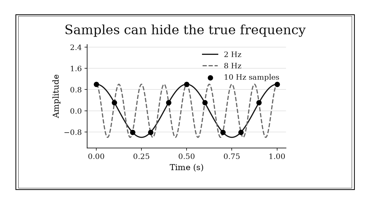
Figure 24.1. Sampling at 10 Hz makes cos(2pi·2t) and cos(2pi·8t) identical at every sample time. An anti-alias filter must remove unwanted high-frequency content before sampling.
24.1.2: Low-pass before every downsampling step
History
Cutting a data stream down to a fraction of its samples is only safe if the discarded fraction never carried anything worth keeping. Ronald Crochiere and Lawrence Rabiner published in October 1975 a design procedure for multistage decimation, lowering a digital signal’s sample rate. Their decimator made a low-pass filter, blocking frequencies above a chosen cutoff, a required stage rather than later cleanup, because discarded samples’ energy above the new, lower Nyquist limit had already folded onto the frequencies that remain.
The equation
For integer decimation factor (M),
where the low-pass response should be strongly attenuated for frequencies that would fold into the retained band, in particular near
How to read it
Keeping every th sample lowers the rate from to and shrinks the safe frequency range, the Nyquist interval, by that factor. A frequency once inside the wide range can sit outside the narrower one, and once samples are discarded, it has already folded onto a lower frequency in the kept data, with no later processing able to separate the two. Filtering after discarding is too late. Nothing in the rule specifies how sharp the filter must be; that depends on how close the wanted band sits to the new Nyquist edge.
How to use it
A seismologist downsamples ground-motion data recorded at Hz by a factor of before archiving. The new rate is Hz and the new Nyquist frequency is Hz. If frequencies worth keeping end at Hz, the filter has a transition band of Hz before decimating. A quarry blast near Hz would otherwise fold to Hz, landing inside the microtremor band the station monitors.
The seismologist uses a tested polyphase decimation routine, specifying ripple, transition width, and stopband attenuation before any sample drops, cascading two stages of rather than one of since the transition is narrow relative to the full factor. This is a Workflow rule: filtering is a required component of the downsampling operation.
24.1.3: Compute FFT bin spacing as sample rate over transform length
History
A faster way to compute a calculation can trick users into thinking the calculation itself changed. Working at IBM’s Yorktown Heights laboratory and Princeton University, James Cooley and John Tukey published, in April 1965, an algorithm computing a fixed set of discrete Fourier frequencies with far fewer operations than direct summation, making large transforms routine. The algorithm made an existing frequency grid cheap to evaluate; it did not move where those frequencies sit. Reading bin as hertz is a modern convention layered on their result, not a claim the paper made.
The equation
For an (N)-sample transform at sample rate (f_s),
With unpadded record duration (T=N/f_s),
How to read it
An FFT (fast Fourier transform) reports a signal’s strength at equally spaced frequencies, called bins, computed from samples taken at sampling rate . Each bin sits hertz above the last; equivalently where is the recording’s length. A denser bin grid does not by itself say whether two close tones can be told apart; that depends on how wide each bin’s underlying window shape is, which can span several bins.
How to use it
A cardiac technician analyzes heart-rate variability from a -second recording sampled at Hz, giving samples and a bin spacing of Hz. Bin represents Hz, the boundary the lab uses to separate low-frequency and high-frequency power bands. The technician labels the spectrum with this formula rather than the software’s default axis, which sometimes plots normalized frequency instead of hertz.
A respiratory peak near Hz and an artifact Hz away will not necessarily separate just because both fall on distinct bins; that depends on the window’s width, not the labeling. The technician escalates to a longer recording before reporting the two as distinct. This is an Independent rule: it gives the exact DFT frequency grid from rate and transform length.
24.1.4: Increase record duration to improve true frequency resolution
History
Padding a recording’s transform with zero samples produces a smoother plot, but tightening a spectral peak this way is an illusion with real consequences for separating two close tones. Working at the Naval Undersea Center in San Diego, Fredric Harris’s January 1978 window survey separated the FFT’s bin width from the wider spectral shape a finite record and its taper impose. His two-tone test varied the taper instead: a sharp window lets a strong tone bury a weak one nearby; a deeper taper uncovers it. The rule’s arithmetic, not his example, says a longer record narrows that shape further.
The equation
To investigate features separated by (f), begin with
The unpadded bin scale is (1/T), while the chosen window multiplies that scale by a main-lobe-width constant.
How to read it
To separate two frequencies apart, observation time needs to be on the order of seconds; the unpadded grid spacing is regardless of zeros later appended. A finite recording multiplies the true signal by a window, a fixed observation shape that stops or tapers at the ends; in frequency, that blurs every sharp line into a shape of finite width. A longer recording narrows the blur. The reciprocal is only a rough scale: window shape, tone loudness, and noise change how much longer the recording needs to be.
How to use it
A music archivist digitizing a wax cylinder suspects the playback motor drifted, splitting the usual Hz hum into components near and Hz, a difference of Hz. The reciprocal separation gives s as a first duration scale for direct Fourier inspection, not an absolute identifiability limit. A Hann taper, chosen for other artifacts, may demand longer than this reciprocal suggests, since one hum is fainter.
The archivist selects a -second segment, above the -second starting scale, rejecting a shorter -second clip whose padded FFT could display two convincing peaks even though its true resolution scale, Hz, is too coarse to support that separation from a Fourier peak plot alone without stronger signal assumptions or independent evidence. This is an Independent rule: it directly links acquired duration to the scale of distinguishable frequency structure.
24.2: Interpret a Spectrum Without Manufacturing Detail
A finite record is already windowed, whether deliberately or by a rectangle. Tapers, padding, and short-time transforms change how the existing information is displayed and estimated. Decibels change its numerical language. None of these operations repeals acquisition limits.
24.2.1: Window noncoherent records before spectral measurement
History
Engineers arguing over which window to apply to a noisy record are usually arguing past each other, because no single taper wins on every count. Fredric Harris’s January 1978 survey, assembled during that same San Diego project, catalogued window shapes and used a two-tone test to show why the choice changes what a transform reveals: a smoother taper lowers distant leakage, energy spreading where it does not belong, at the cost of a wider peak, while a sharper-edged one leaks further but stays narrow. Harris tabulated these tradeoffs rather than naming a winner.
The equation
Window the acquired record as
Multiplication in time gives convolution in frequency:
up to the transform’s normalization convention.
How to read it
Multiplying a recorded segment by a window, a weighting shape applied before the transform, is unavoidable: even cutting a recording off at its edges applies a rectangular window with abrupt endpoints. That abruptness produces leakage, a tone’s energy spreading into nearby frequencies. A smoother taper such as a Hann window suppresses that spreading, at the price of a wider true peak. The rule does not say which taper to pick; that choice trades leakage suppression against a wider true peak. Windowing also changes a tone’s measured amplitude, its coherent gain, needing correction for whichever window is chosen.
How to use it
A vibration analyst records second of accelerometer data from a conveyor bearing at a rate giving Hz bin spacing, and finds a suspected defect tone near Hz, a half-bin offset of Hz. Under a rectangular window, the offset spreads the tone’s energy across neighboring bins as leakage, burying a second, weaker defect tone near Hz. A Hann window suppresses the leakage enough to expose it, at the cost of a broader peak.
The analyst corrects coherent gain and accounts for the tone’s half-bin offset, for example by fitting its frequency and evaluating the windowed transform there. Coherent-gain correction alone leaves Hann’s nearest-bin scalloping loss, about 1.42 dB at a half-bin offset, and nearby-tone leakage still needs checking. This is a Workflow rule: it selects and normalizes a taper as part of spectral measurement.
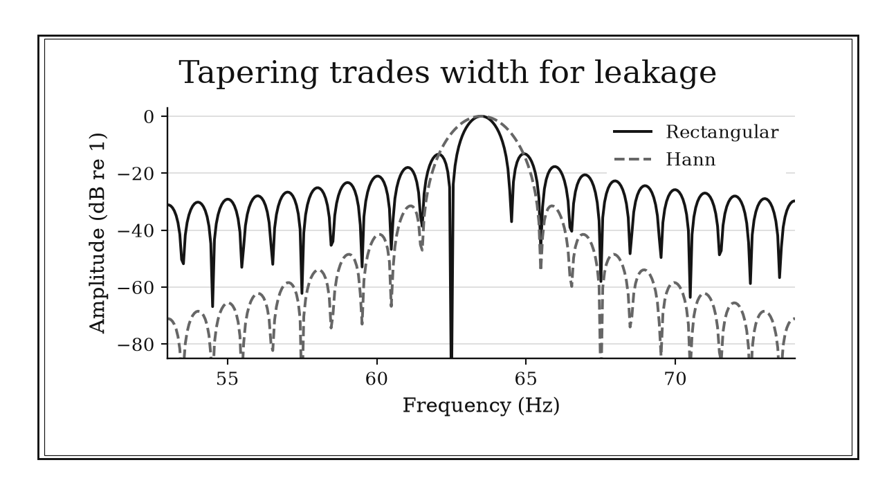
Figure 24.2. A one-second, 63.5 Hz tone leaks into distant frequencies under a rectangular window. A Hann taper suppresses sidelobes but broadens the main lobe. Dividing by each window’s sum corrects coherent gain.
24.2.2: Use zero padding for spectral interpolation, not added resolution
History
Can a spectrum be made to look sharper just by asking a computer to plot more points from it? Working between Vancouver, British Columbia and Edmonton, Alberta, Mauricio Sacchi, Tadeusz Ulrych, and Colin Walker developed a 1998 high-resolution method for spectral estimation and data extrapolation. Setting up their approach, they identified ordinary zero padding, appending zeros before transforming, as the standard way to obtain more spectral samples, noting that padding alone does nothing to narrow the sidelobes fixed by the record’s finite length. Their extrapolation method added resolving power through added assumptions; plain padding adds none.
The equation
Padding (N) acquired samples to transform length (K>N) gives
The plotted spacing becomes (f_s/K), but the acquired duration remains (N/f_s) and the window lobe remains tied to that duration.
How to read it
Zero padding appends zeros to a recorded segment before computing its transform, lengthening the calculation without lengthening the observation. The unpadded segment already defines one continuous curve in frequency; padding to a longer length reads more points off that curve, at spacing , rather than acquiring new information. The curve’s shape, how wide each true peak is, stays fixed regardless of padding. Padding can still sharpen a single isolated tone’s location estimate under a good model; that is estimation from data in hand, not resolving power for nearby, unmodeled tones.
How to use it
A hydrophone array operator studying shipping noise records s at Hz, giving samples and an unpadded grid spacing of Hz. Zero padding to plots values every Hz, a smoother curve. Two engine-harmonic tones Hz apart have not become resolvable just because the displayed grid is ten times denser: the acquired record’s ordinary Fourier resolution scale remains Hz.
The operator instead extends the acquisition to s, a genuine spacing of Hz matching the separation: that is a starting resolution scale, and the operator checks the window, amplitude ratio, noise, and actual two-tone separation before reporting distinct components. This is a Workflow rule: it is a display and interpolation operation whose limits must remain attached to the acquired record.
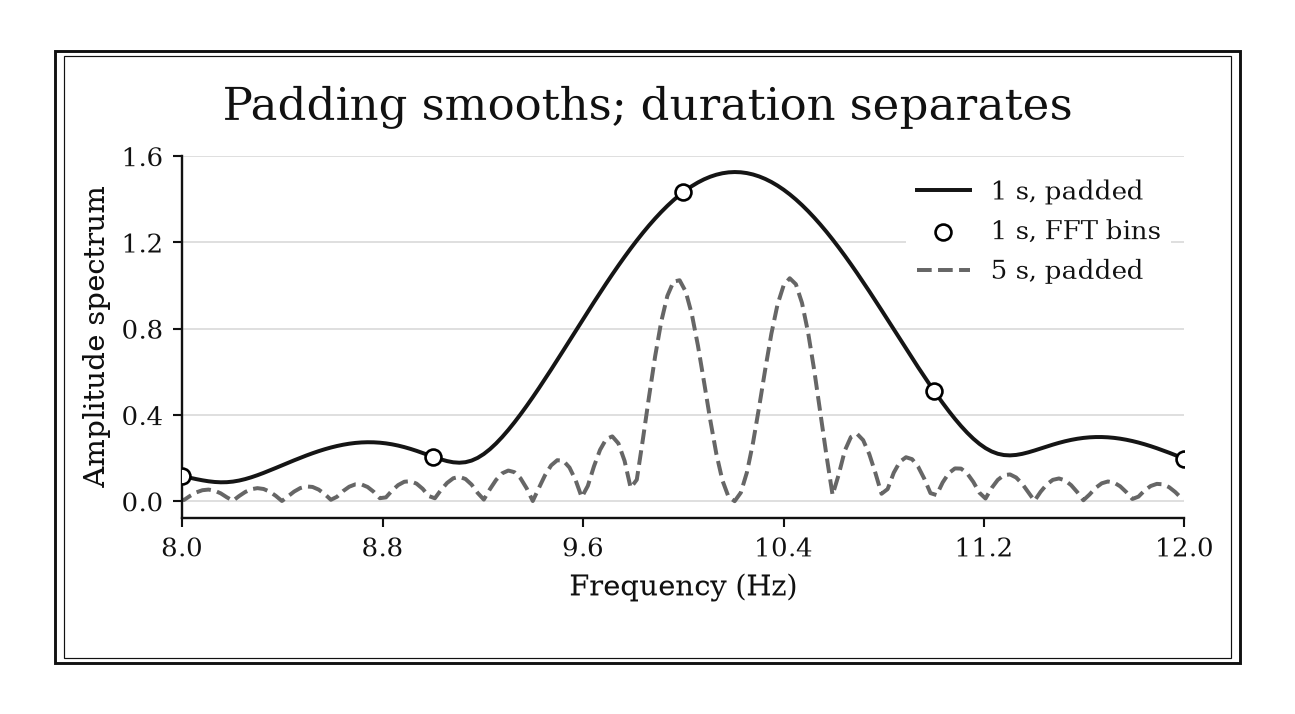
Figure 24.3. Two constructed tones at 10 and 10.4 Hz blend in a one-second record even after zero padding. A five-second record contains more resolving information. All spectra use rectangular windows and amplitude normalization by acquired length.
24.2.3: Choose STFT window from the shortest event and closest tones
History
A cell bounded in both time and frequency, rather than a pure, endlessly repeating wave, is the basic building block Dennis Gabor proposed in November 1946 for representing communication signals. Working at the British Thomson-Houston Research Laboratory in Rugby, Warwickshire, Gabor drew on quantum-mechanical uncertainty to argue that frequency content should never be treated as detached from when it occurred. That construction is a direct ancestor of the short-time Fourier transform; its core tension, tightening a cell in time widens it in frequency, is what any STFT window length negotiates.
The equation
For an STFT window of duration (T_w),
where constants depend on window definition and on what “resolved” means.
How to read it
A short-time Fourier transform (STFT) slides a window of fixed duration along a recording and computes a spectrum from each slice. A short window tracks fast events in time, roughly to within , but its Fourier transform is broad, giving frequency resolution only around . A long window narrows that scale but blurs anything changing within its span. Overlapping windows more densely changes how many time frames get reported, smoothing output, but does not create new, independent information beyond one window’s data.
How to use it
A bridge-monitoring technician tracking acoustic-emission bursts on a highway bridge, brief clicks indicating microcracking, needs to both time-locate bursts and separate two traffic-induced resonance tones Hz apart. A ms window localizes a burst to roughly that duration but has a frequency scale near Hz, far too coarse for the tones. Lengthening to s improves the scale to Hz, matching the separation, but smears exactly when within that s a burst occurred.
The technician runs both window lengths, the short one to log burst timing and the long one to confirm the resonance split, rather than assuming one setting delivers both answers. This is a Workflow rule: it selects a local analysis scale by exposing an unavoidable time-frequency compromise.
24.2.4: Twenty decibels means tenfold amplitude or hundredfold power
History
Adding up the loss and gain of dozens of cable sections by multiplying ratios together is exactly the bookkeeping telephone engineers could not afford to get wrong. Bell System engineers replaced an older unit, the mile of standard cable, with a logarithmic transmission unit in 1923, and deliberations begun in 1924 later recommended the names bel and neper. In the January 1929 Bell System Technical Journal, W. H. Martin documented the Bell System’s adoption of decibel for the unit. The scale was built on power ratios; the amplitude version follows algebraically from power proportional to amplitude squared, not a rule Martin stated separately.
The equation
For power,
If (P=C|A|^2) with the same (C),
How to read it
A decibel (dB) expresses a ratio on a logarithmic, multiply-becomes-add, scale rather than an absolute quantity. A dB power increase means the power ratio is . The same dB also describes an amplitude ratio of whenever power is proportional to that amplitude’s square under matching reference and loading conditions: two readings of one change. A bare dB number is just a ratio; units like dBm or dB SPL add a reference level. Whether a dB change sounds twice as loud is a separate question this arithmetic does not answer.
How to use it
A telecom line engineer measures a test tone’s RMS voltage across a repeater section, both readings taken over the line’s standard impedance: V in, V out. The voltage ratio is , giving dB. Power in is mW; power out is mW, a ratio of , and dB confirms the gain.
If the V reading came instead from a mismatched point, power there is mW, a ratio of only , giving dB, not . The engineer records impedance alongside every reading. This is an Independent rule: it directly converts compatible power and amplitude ratios across many applications.
24.3: Estimate Spectra and Implement Filters Safely
Spectral estimates are random quantities, and filters are numerical realizations rather than symbolic transfer functions. Segment length, overlap, window bandwidth, section form, and data direction all change what an implementation means.
24.3.1: Trade Welch segment length against PSD variance
History
A power spectral density from one transform is a single noisy sample, not a settled truth: repeat the acquisition and the peaks can shift. Peter Welch, working at the IBM Research Center in Yorktown Heights, New York, published in June 1967 a method splitting a record into possibly overlapping segments, windowing and transforming each, then averaging the resulting periodograms, each a single-record power spectrum estimate. He made the exchange explicit: shorter segments produce more averages and calmer output, longer segments finer frequency detail but a noisier curve.
The equation
For segment length (N_{seg}),
If (K_{eff}) effectively independent modified periodograms are averaged, relative random error scales roughly as
How to read it
A power spectral density (PSD) estimate is not a fixed curve; it is a noisy quantity a single transform does not settle. Averaging several estimates reduces that noise. For a fixed recording length, shortening each segment to samples widens the frequency scale to roughly but allows more segments to average; averaging roughly independent segments shrinks relative random error by about . The count of segments run is not automatically the effective number of independent averages: overlapping segments are correlated, so counting them overstates how much noise has really been beaten down.
How to use it
A radio astronomer has a -second baseband recording and must choose a Welch segment length before searching for a faint spectral line near a strong interference tone. Splitting into -second segments gives averages and a scale near Hz, stabilizing the noise floor. Splitting into -second segments gives only averages but sharpens the scale to Hz.
The astronomer starts from the narrowest feature that must stay visible, a line about Hz wide, and picks the -second segmentation despite its rougher floor. Because receiver gain drifted during the recording, segments from opposite ends are not comparable, so averaging stays within segments recorded close together. This is a Specialized rule: it tunes an internal PSD estimator by balancing resolution and variance.
24.3.2: Start Welch averaging with Hann windows and fifty-percent overlap
History
Skip overlap entirely with a Hann-windowed record, and the samples a Hann window already downweighted near each segment’s edges get counted only once, never recovered at full strength. In a January 1978 study building on Peter Welch’s earlier recommendation of half-length overlap, Fredric Harris measured the correlation between successive windowed transforms at 50 and 75 percent overlap, part of the same San Diego survey. He found that at 50 percent, transforms computed with a good window were essentially independent, recovering most of the variance reduction nonoverlapping segments were forfeiting.
The equation
For Hann-windowed segments, begin with
With record length (N), hop (H=N_{segment}-N_{overlap}), the full-segment count is
How to read it
Overlap is how much of one segment’s samples are shared with the next; fifty-percent overlap means each new segment reuses half the samples from the one before it. A Hann window gives little weight to a segment’s own edges, so shifting the next segment by half a length lets those edge samples contribute again, nearer the center of a different window, at full weight. More transforms become available from an unchanged recording, helping average down noise. Piling on overlap is not guaranteed to keep paying off at the same rate: past fifty percent, extra transforms yield diminishing extra information.
How to use it
A power-quality engineer captures a -sample record of grid voltage to check harmonic distortion and divides it into -sample Hann-windowed segments with -sample overlap. The segment count works out to
compared with only segments with no overlap, nearly doubling the averages from the same captured cycles.
The engineer reports amplitudes using the software’s Hann-consistent normalization, logging sample rate, segment length, and overlap, since mismatched settings would compute a different noise floor from identical raw samples. More overlap, say 87.5 percent, adds strongly correlated segments and may bring a small further variance reduction, but neither the seven segments nor the larger count should be treated as fully independent averages. This is a Specialized rule: it supplies a practical initial configuration inside Welch averaging.
24.3.3: Use equivalent noise bandwidth when converting FFT noise to density
History
Identical bin spacing on two spectra does not fix how many hertz of noise each bin represents; that number can differ, correctly, between readings. The same window catalog, a January 1978 comparison, saw Fredric Harris tabulate measurable window properties rather than rank tapers by name, defining equivalent noise bandwidth as the width of an ideal rectangular filter passing the same broadband noise power as the real window. His split between coherent gain, a tone’s response, and incoherent power gain, noise’s response, explains why dividing noise by bin width alone is often wrong.
The equation
For window samples (w[n]),
and
How to read it
Equivalent noise bandwidth (ENBW) is the width, in bins or hertz, of an ideal flat-topped filter collecting the same broadband noise power as the actual window. It comes from two sums of the window’s sample values: the sum of squares sets noise power passed, the plain sum how strongly a tone comes through. ENBW is usually wider than one bin, so measured noise must be spread over that wider bandwidth, not the nominal spacing, when converting to a density. It assumes noise is roughly flat across that bandwidth, and applying it twice by mistake is easy, since PSD software often already includes it.
How to use it
A wind-turbine reliability engineer records samples of gearbox vibration at Hz, a bin spacing of Hz. Analyzing with a periodic Hann window, whose equivalent noise bandwidth is about bins, means each noise bin integrates Hz of vibration energy, not Hz.
Converting the noise floor into a density against the manufacturer’s spec requires first confirming whether the software’s PSD scaling already applies this correction; skipped, dividing by Hz instead of Hz overstates the reading by , possibly flagging a healthy gearbox as exceeding its limit. This is a Specialized rule: it performs the normalization step needed for quantitative FFT noise density.
24.3.4: Implement moderate-to-high-order IIR filters as second-order sections
History
Why can a tenth-order filter written as one long polynomial behave nothing like the same filter written as five smaller pieces, when the two are algebraically identical? Leland Jackson analyzed roundoff noise, small errors from rounding numbers to a fixed number of digits, in fixed-point filters realized in cascade and parallel forms, in June 1970. His calculations went further than comparing symbolic transfer functions: he examined how pole-zero pairing and section ordering changed numerical behavior, and supplied practical rules for choosing both.
The equation
Factor a filter as
Each factor is a biquad; real filters pair complex-conjugate poles and zeros into real-coefficient sections.
How to read it
An IIR (infinite impulse response) filter of moderate or high order, meaning many pole-zero pairs, can be written as one long numerator and denominator, or as a cascade of low-order second-order sections. Multiplying many roots, the numbers that set where the filter rings and how sharply, into one polynomial can make its coefficients extremely sensitive: a tiny rounding error can move a root when poles cluster for a narrow band. Second-order sections keep that sensitivity local, letting each section’s values be rescaled independently. The form does not guarantee safe behavior; overflow, an internal value exceeding the number format’s range, and instability remain possible.
How to use it
An automotive noise-and-vibration engineer designs a tenth-order Butterworth filter for active noise cancellation and factors it into second-order sections rather than one polynomial, inspecting every pole’s radius against the processor’s actual fixed-point precision.
Placing the highest-gain section first can let its output exceed the number format’s range even though the overall response stays bounded, corrupting every section downstream. The engineer tests orderings and gain scaling of the sections against worst-case inputs, checking peak internal states as well as the overall output. This is a Specialized rule: it changes the numerical realization stage of an IIR design without changing the intended transfer function.
24.3.5: Use forward-backward filtering only for offline zero-phase work
History
Run the same forward-backward filter on a recording twice, once forward-then-back and once back-then-forward, and the two traces do not have to agree at their ends. Fredrik Gustafsson, working at Linköping University, studied that defect in April 1996: arbitrary initial-state choices produce different transients at the two ends of a finite record. He derived states making forward-backward and backward-forward processing agree more closely, addressing a finite recording’s boundary conditions, not a way to run the operation causally, in real time.
The equation
For a real-coefficient one-pass response (H),
The phase cancels, while the magnitude response is squared and the effective filter order doubles.
How to read it
Forward-backward filtering, often called zero-phase filtering, runs a signal through a filter once forward and once in reverse. Reversing time flips the sign of a filter’s phase delay, so the second pass cancels the timing shift the first introduced; but the magnitude responses multiply, so attenuation applies twice and the combined response has twice the one-pass filter order; this does not mean a finite number of samples determines an IIR filter’s memory. The backward pass needs data from later in the record, so the operation is noncausal. Good initial states, as Gustafsson worked out, still leave zero phase short of zero edge error: finite records need an explicit endpoint treatment, such as padding or a suitable initial-state method, and edge contamination can remain.
How to use it
A sports biomechanist analyzing a -sample accelerometer trace of a jump landing wants offline smoothing without one-pass phase delay, so considers a forward-backward filter. Zero phase does not guarantee an unchanged threshold-based ground-contact time, which must be checked against the event definition. A one-pass Butterworth filter set to dB at its cutoff becomes dB once applied both ways, so the filter is designed for a higher cutoff than the desired final point.
The trace is only samples and the filter’s memory spans roughly , so the first and last samples of the output are discarded from the timing measurement: the interior must still be checked for event-time changes caused by waveform smoothing, and the discarded edge length must be validated for this filter and record. This is a Workflow rule: it selects a whole-record operation whose magnitude, causality, and endpoint costs must be accepted together.
Chapter Synthesis: Preserve the Difference Between Information and Display
Sampling rate protects the wanted band from aliases, while record duration determines a basic separation scale. Those are acquisition choices. Anti-alias filtering must precede every lower-rate representation, and FFT bin labels must come from the actual sample rate and transform length.
Windows, padding, and STFTs reorganize a finite record. A taper controls leakage by widening its spectral response. Padding interpolates that response without narrowing it. A short-time window trades event localization against tone separation. Decibels compress ratios only after the correct power, amplitude, impedance, and reference conventions are identified.
Spectral estimation and filtering add implementation contracts. Welch averaging trades segment length against random variance. Hann overlap reuses downweighted samples without manufacturing independence. ENBW normalizes broadband noise. SOS protects IIR roots in finite precision. Forward-backward filtering cancels phase only by becoming offline, squaring magnitude, and confronting endpoints.
Across all thirteen rules, ask:
- Was the needed information acquired at a sufficient rate and duration before processing began?
- Does an operation add evidence, or only interpolate, taper, average, or relabel existing evidence?
- Are amplitude, power, PSD, bandwidth, reference, and impedance conventions explicit?
- Is the implementation causal and numerically stable in the precision actually used?
One-Page Signal Processing Toolkit
| Recognition cue | Rule to try | What it gives | Role |
|---|---|---|---|
| Highest wanted analog frequency known | Sample above twice it with filter transition room | Acquisition-rate floor | Independent |
| Sample rate will decrease | Low-pass before discarding samples | Alias protection | Workflow |
| FFT index needs physical units | Use (f=f_s/N=1/T) | Exact bin grid | Independent |
| Two close tones must separate | Increase acquired duration | True resolution scale | Independent |
| Record is not coherent | Choose and normalize a taper | Leakage control | Workflow |
| Plot needs more frequency samples | Zero-pad while preserving original duration | Spectral interpolation | Workflow |
| Signal changes over time | Choose STFT window from events and tones | Local analysis scale | Workflow |
| Gain or loss is reported in dB | Distinguish (10) power from (20) amplitude | Linear ratio | Independent |
| PSD is too noisy | Trade Welch segment length against averages | Resolution–variance budget | Specialized |
| Welch configuration needs a default | Hann with 50% overlap | Practical starting setup | Specialized |
| FFT noise must become density | Apply window ENBW | Correct noise bandwidth | Specialized |
| IIR order is moderate or high | Cascade second-order sections | Stable realization | Specialized |
| Offline timing must not shift | Forward–backward filter with edge checks | Zero-phase whole-record result | Workflow |
Decision Path
- Are analog or preexisting digital components above the new Nyquist limit? Filter before sampling or decimation; after folding, recovery is not generally possible.
- Is the question about bin labels or resolving components? Use (f_s/N) for labels and acquired duration plus window width for resolution.
- Does a tone fail to land on a bin? Choose a taper, correct coherent gain and off-bin scalloping for tone amplitude, and apply ENBW only when the noise-density scaling requires it.
- Does a denser spectrum look more detailed? Check whether new samples were acquired or only zeros were appended.
- Does the signal change in time? Select STFT windows against both event duration and tone spacing; use more than one scale when necessary.
- Is a level stated in decibels? Identify power versus amplitude, reference level, impedance, and one-sided or RMS conventions before converting.
- Is a PSD unstable? Vary Welch segment length, quantify effective averaging, and report confidence rather than hiding variance with overlap.
- Is a filter high order or zero phase? Use SOS for numerical realization and reserve forward–backward application for offline records with explicit edge treatment.
Transfer Problems
1. Design a rate conversion
A sensor records at (96) kHz, contains wanted content through (8) kHz, and must be stored at (24) kHz. State the new Nyquist limit, choose a plausible transition band, identify when filtering occurs, and predict where an unfiltered (18) kHz component would alias.
2. Separate grid density from resolution
One second of data is sampled at (2000) Hz and padded from (N=2000) to (K=20{,}000). Compute both plotted spacings, state the acquired resolution scale, and explain what must change to distinguish tones at (100.0) and (100.2) Hz.
3. Build a quantitative PSD and filter workflow
For a (4096)-sample record at (1024) Hz, choose Hann-Welch segments and overlap, calculate the segment count and frequency scale, include ENBW in a noise-density conversion, and explain why a tenth-order IIR should use SOS and why its forward–backward version cannot run live.
Where These Ideas Reappear
- Ordinary differential equations: points per oscillation and phase error parallel sample-rate and window-resolution decisions.
- Partial differential equations: cells per wavelength, artificial boundaries, and numerical dispersion mirror finite-record spectral effects.
- Control theory: sampling, delay, gain margins, sensor noise, and causal filters turn signal-processing choices into stability costs.
- Statistics: Welch averaging, effective degrees of freedom, and confidence intervals are variance-estimation problems.
- Information theory: sampling limits, channel bandwidth, and logarithmic ratios determine how much distinguishable information can be conveyed.
- Scientific computing: SOS conditioning, normalization conventions, and reproducible metadata are numerical implementation contracts.
Historical Notes and Sources
All thirteen profiles have verified historical stories. The chapter distinguishes ideal reconstruction theorems and documented algorithms from later guard bands and practical numerical defaults.
- Shannon, Nyquist, and sampling: Shannon’s original 1949 paper; Nyquist’s 1928 transmission paper.
- Crochiere and Rabiner on decimation: original IEEE paper; National Diet Library record.
- Cooley and Tukey’s FFT: original paper; IBM Research record.
- Harris on windows, duration, overlap, and ENBW: original 1978 paper; MIT-hosted copy.
- Sacchi, Ulrych, and Walker on interpolation versus extrapolation: original IEEE paper; University of Alberta copy.
- Gabor and time-frequency atoms: original 1946 paper; Royal Society memoir.
- Martin and the decibel: Nokia Bell Labs archive; original 1929 journal scan; NIST SI guidance.
- Welch and averaged periodograms: original 1967 IEEE paper; Harris’s overlap analysis.
- Jackson and digital-filter realization: original 1970 IEEE paper; NASA memorandum on modern SOS use.
- Gustafsson and forward–backward initial states: original IEEE paper; Linköping University record.
- Modern formulas and API conventions: SciPy signal-processing reference; SciPy Welch reference; Smith, Spectral Audio Signal Processing; ITU-T Recommendation B.12.