Chapter 25: Control Theory: Performance, Robustness, and Implementation Reality
A controller can look excellent in a continuous-time simulation and oscillate as soon as it is deployed. One sample of computation delay, a saturated actuator, a noisy derivative, or an omitted fast pole can spend the phase and gain reserves that made the nominal design appear comfortable.
Feedback design is therefore a budget, not a single tuning calculation. Bandwidth buys speed but raises exposure to delay, sampling, noise, and unmodeled dynamics. Integral action removes constant offset but creates windup when authority runs out. Classical margins summarize useful geometry, yet sensitivity and nonlinear implementation checks are needed to decide whether the loop remains credible away from its nominal model.
The ten rules in this chapter form three themes. The first translates desired behavior into bandwidth, integral structure, and dominant modes. The second protects robustness at crossover through phase margin, gain margin, and peak sensitivity. The third charges delay, digital sampling, saturation, and derivative noise against the design.
The governing habit is: turn every performance improvement into an explicit robustness and implementation cost before closing the loop.
25.1: Translate Desired Behavior Into Loop Structure
Time-domain requirements suggest frequency scales, while disturbance classes suggest controller structure. Reduced pole models can simplify design, but only after the discarded dynamics have been shown to decay fast enough and contribute little enough.
25.1.1: Estimate rise time from closed-loop bandwidth
History
Adjust a 1940s feedback amplifier and the only way to know its new speed was to grind out the full time response again; guess instead, and the design misled you. Hendrik Bode broke that bottleneck in 1945 at Bell Telephone Laboratories in New York with Network Analysis and Feedback Amplifier Design, turning gain and phase into a frequency-based design language for judging bandwidth, stability, and transient speed. Bode’s book stops at the frequency-based design language. The rise-time-times-bandwidth coefficient is an engineering fitting, tuned to response shape and to how rise time and bandwidth get defined.
The equation
Write the scale consistently as
for common well-damped low-order responses. A first-order 10–90% rise has (c=), so
How to read it
is rise time: how long the closed loop takes to climb from 10% to 90% of a step’s height. is closed-loop bandwidth in radians per second, the fastest rate the loop can follow a change; is the same corner in hertz. The rule treats them as reciprocal partners: multiply rise time by bandwidth and the product sits near 2, not a fixed number. A 10 Hz bandwidth loop turns in a rise time near 35 milliseconds. The coefficient shifts with damping, extra zeros, higher poles, and which transfer function was measured, so treat it as a starting scale, not a guaranteed reading.
How to use it
A flight-test lead needs a commanded tilt to have a 10-90% rise time of about 0.2 seconds, quick enough to catch a gust before it tips the frame.
about 1.4-1.8 Hz; the lead targets 10 rad/s (about Hz) and moves to bench testing.
The bench step response has a 10-90% rise time longer than 0.2 seconds because propeller dynamics add an extra pole the ratio never saw. The lead separately checks overshoot and settling time, which the rise-time estimate does not specify. Simulating the actual response, not the estimate, catches that gap before the drone does. This is an Independent rule: it directly converts a speed requirement into an initial bandwidth scale while labeling its approximation.
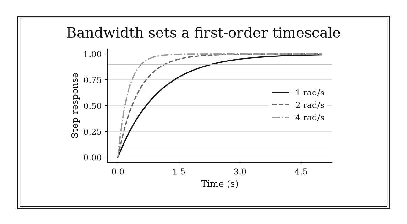
Figure 25.1. For first-order closed loops, 10-to-90 percent rise time is ln(9)/omega_BW. Doubling bandwidth halves rise time in this model; additional poles or zeros can change the relation.
25.1.2: Add integral action for zero steady-state error to constant disturbances
History
A ship steering only on proportional correction settles into a permanent heading error against a steady crosswind, because proportional action needs a nonzero error to produce a nonzero correction. Nicolas Minorsky worked out why in May 1922, publishing “Directional Stability of Automatically Steered Bodies.” He formalized the actions now called proportional, integral, and derivative, writing down what a skilled helmsman did by feel. The internal-model explanation of why correction cancels a constant bias came later; the payoff was Minorsky’s: a growing rudder command erases an error a proportional-only rudder never could.
The equation
Integral action contributes
For loop transfer (L) and sensitivity (S=1/(1+L)), a stable loop with uncancelled integral gain has
How to read it
says the integral term’s output keeps climbing while any error remains, at a rate set by gain . is the loop’s total gain and is sensitivity, how much of a disturbance survives into the output. Push at zero frequency toward infinity and is squeezed toward zero: a constant error gets rejected completely at steady state, the way a thermostat keeps nudging heat up until the room holds. The rule needs the loop to stay stable and the actuator to have authority left; a disturbance that keeps changing, like a ramp, sits outside what it cancels.
How to use it
A building engineer running a proportional-only heater watches the room settle 2 degrees below setpoint every cold night, because steady heat loss needs a nonzero error to keep the heating command above zero. Adding integral action lets that error accumulate until delivered heat matches the loss. With integral action the loop gain at zero frequency grows without bound, so the surviving fraction of the disturbance is : the 2-degree offset goes to zero. The engineer tunes for margin and speed.
If the heater already runs near full output, the growing integral command has nowhere to go, a saturation problem integral action alone cannot fix. Testing startup and worst-case load first protects against that. This is a Workflow rule: it selects controller structure from the disturbance class and offset requirement.
25.1.3: Trust a dominant-pole approximation only with clear separation
History
Two engineers can disagree about whether a distant pole is safe to drop from a design. Walter R. Evans presented the root-locus method in New York in early 1950, letting that disagreement be checked directly: his plot traced every closed-loop root as gain changed, so a pole dropped from a simplified model reappeared on the same drawing. The rule that a pole five times farther left than the dominant pair can usually be ignored is later heuristic guidance built on Evans’s framework, not a claim Evans made himself.
The equation
For stable poles, a starting separation test is
Modal terms behave like
so both pole location (p_k) and residue (r_k) matter.
How to read it
is the pole, a decay rate, kept in a simplified model; is a candidate pole left out. is the decay rate: a mode behaves like , dying out at a speed set by and a size set by residue . A fast pole five times farther left decays about five times sooner, the way a sprint finishes long before a marathon’s halfway mark. A large residue can make that mode loom large at the start, and a pole near a zero can stay fragile despite passing the fivefold test.
How to use it
A water-utility operator is deciding whether a pump model with a fast electrical pole can be replaced by a simpler second-order model for pressure-loop tuning. Poles sit near and the candidate to drop sits at :
clearing the separation test, so the reduced model looks safe to tune against.
The operator still compares full and reduced step responses rather than trusting location alone. If the true fast pole were at instead, falls short of 5 and the reduced model could mislead the tuning. This is a Workflow rule: it guards model reduction by checking both timescale separation and modal influence.
25.2: Protect Robustness at Crossover
Classical margins measure how far a simple loop is from critical Nyquist geometry under selected perturbations. They are useful starting screens, not universal certificates. Peak sensitivity adds a direct distance measure around the entire frequency path.
25.2.1: Start loop shaping near 45 to 60 degrees phase margin
History
How much extra lag can a feedback loop tolerate before it starts to oscillate on its own? Harry Nyquist answered that question in January 1932, at the same laboratory, encoding the whole feedback loop as a curve in the complex plane and reading stability from its relation to one critical point. His construction gave the phase remaining at unit loop gain a direct stability meaning: a measurable reserve against added lag. The 45-60 degree phase-margin band belongs to postwar design handbooks built on that geometry; Nyquist’s paper specified no target.
The equation
At gain-crossover frequency (_c), where
phase margin is
under the conventional negative-feedback sign.
How to read it
is the loop transfer function, the combined gain and phase of the feedback path; is the crossover frequency, where equals 1. Phase margin measures how much added lag would pile up at that crossover before the loop rotates to the unstable direction. More margin usually buys smoother, better-damped behavior, the way extra following distance forgives a slow reaction. That reading depends on one clean crossover; a second crossing or an unstable open-loop pole changes what the number guarantees.
How to use it
An automotive engineer tuning a cruise-control loop measures the loop’s phase at where its magnitude crosses 0 dB, giving
inside the usual 45-60 degree range. The engineer charges the throttle actuator’s and sensor’s known delay against that reserve and inspects the closed-loop step response for overshoot.
If the vehicle later gets a slower, cheaper throttle actuator, the added delay eats into those 50 degrees while the previously computed nominal margin remains on the design sheet, so a design comfortable on paper can shudder on the road. Checking all crossings and a nonlinear simulation with the real actuator catches what one scalar margin cannot. This is a Workflow rule: it supplies a robustness target within a larger frequency-domain design and verification process.
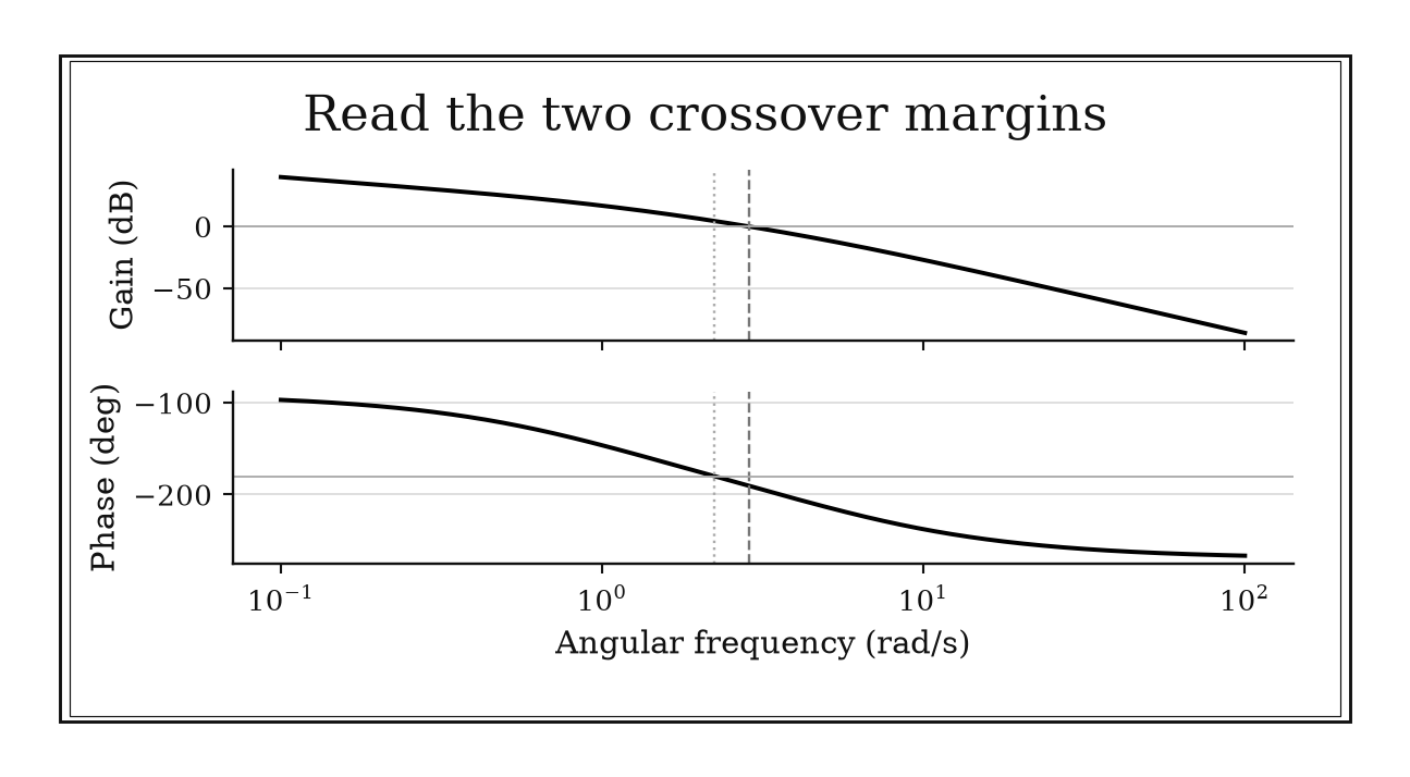
Figure 25.2. For the constructed loop L(s)=10/[s(1+s)(1+s/5)], phase margin is about -10.5 degrees and gain margin about -4.4 dB. Both margins warn of the unstable closed loop; a familiar Bode shape alone is not a certificate.
25.2.2: Seek at least about 6 dB classical gain margin
History
Where phase margin reads a loop’s angle at crossover, gain margin reads the same Nyquist curve’s distance from the critical point, along the radius rather than around the angle. That radial reading answered directly, without testing an amplifier bench by bench, how much its gain could rise before a stable feedback loop tipped into oscillation. Nyquist’s geometry drew the picture; the “about 6 dB” target came later, as engineering convention.
The equation
At a phase-crossover frequency (_{pc}) satisfying
define
Six decibels is approximately a factor of two in loop gain.
How to read it
is the phase-crossover frequency, where reaches . There, ordinary negative feedback has rotated to act like positive feedback, so whatever gain remains decides whether the loop stays stable. Gain margin is the factor by which loop gain could rise before reaching that point; in decibels, , and 6 dB is roughly doubling the gain. Gain dropping instead of rising sits outside what this margin screens, and if the loop never reaches , software may report an infinite margin that is no safety certificate.
How to use it
A brewery’s fermentation-temperature control loop, plotted on a Bode chart, shows loop magnitude at dB when phase reaches . In decibels that is , so
clearing the usual 6 dB, factor-of-two screen before the brewmaster signs off on the cooling-jacket controller.
That design might still carry a thin phase margin or a large sensitivity peak the gain-margin number alone hides. The brewmaster checks every phase crossing and both directions of gain change, since the chiller can lose capacity as well as gain it, before trusting the batch to run unattended overnight. This is a Workflow rule: it checks one classical robustness direction inside a broader loop assessment.
25.2.3: Keep peak sensitivity near or below two when feasible
History
A spacecraft that points its instruments a fraction of a degree off target can turn a costly observation into unusable data. That stake sat behind a 2010 report to the AIAA Guidance, Navigation, and Control Conference in Toronto, where Mike Ruth, Ken Lebsock, and Neil Dennehy described retuning NASA attitude-control loops using Bode’s sensitivity integral. Pushing bandwidth higher forced sensitivity up elsewhere, a waterbed effect; the report tabulated a peak sensitivity near 1.92 alongside a gain-margin bound near 6.4 dB, giving near 2 a practical screening scale.
The equation
For an internally stable negative-feedback loop with loop transfer (L),
A starting target (M_s) corresponds to no more than about (6) dB peak amplification.
How to read it
is sensitivity: the transfer from an additive output disturbance to the output in the standard unity-feedback arrangement. Other disturbance locations and uncertainty models use different transfer functions. is the worst-case value of across every frequency. Geometrically, is the reciprocal of how close the loop’s curve passes to the critical point ; a high peak means the curve grazes close to instability, even if margins elsewhere look fine. Keeping near or below 2 caps that worst amplification near 6 dB, provided internal stability has first been established; a bounded frequency curve alone cannot establish it. Pushing sensitivity down in one band can force it back up elsewhere.
How to use it
A biomedical engineer tuning an insulin-pump loop against blood-glucose readings compares two controllers with similar phase margin. The first has , so its worst-frequency amplification is
modest even at its roughest frequency. The second has , passing much closer to the critical point and deserving a harder look first.
The engineer plots sensitivity and complementary sensitivity separately, because sensor noise and delivery disturbance travel different channels, and a good on one can hide a bad one on the other. The target of 2 is a heuristic: a genuinely slow physiological response may force a larger peak. This is a Workflow rule: it adds a global frequency-domain robustness diagnostic to classical margins.
25.3: Pay the Delay, Sampling, Saturation, and Noise Costs
The implemented loop contains timing and nonlinearities absent from an ideal block diagram. Delay spends phase without reducing magnitude. Sampling adds hold behavior. Saturation breaks the designed linear loop, and ideal differentiation gives unbounded high-frequency gain.
25.3.1: Convert every delay into phase lag at crossover
History
Delay changes phase without touching magnitude, letting a loop that looks perfectly stable on a magnitude plot fail once real transport time enters the picture. Nyquist’s 1932 contour test judged stability from the whole path a loop traces in the complex plane, the framework a pure delay needs: its magnitude stays at 1 while its phase keeps rotating, so delay drains stability reserve invisibly on a magnitude-only reading. That is the engine behind every delay budget charged against phase margin today.
The equation
A pure delay () contributes
whose frequency response has phase
How to read it
A pure delay of length contributes , whose frequency response has magnitude exactly 1 at every frequency and phase radians, or degrees. Because that phase cost grows with frequency , the same delay is nearly harmless in a slow loop and decisive once the loop speeds up: pure computation and transport delays add through . Sensor filters and actuator dynamics contribute their actual frequency-response phase and can also change magnitude and crossover, so their time constants cannot generally be treated as pure delays. This treats delay as one fixed number; jitter and distributed delays need more careful accounting than a single .
How to use it
An engineer commissioning a building’s HVAC air-handling loop runs crossover at rad/s, then discovers the damper actuator communicates over a wireless network link carrying a 10 ms round-trip delay. That delay costs
of phase margin. A nominal margin, computed before the network was in the loop, leaves only about once the delay is charged against it.
The building’s bench tests, run over a wired connection with negligible delay, showed a margin the deployed, networked system does not have. The engineer measures the real latency on the deployed hardware and lowers crossover rather than trusting the bench number. This is a Workflow rule: it converts implementation timing into a recurring phase-budget component.
25.3.2: Sample a digital control loop at least ten times faster than bandwidth
History
Remove an aircraft’s mechanical control linkage entirely, and every delay in its digital computer’s sampling stops being bookkeeping and starts being part of the airplane’s own dynamics. NASA tested that on May 25, 1972, when Gary Krier flew a modified F-8C in Edwards, California, using an Apollo digital computer as the aircraft’s primary flight controller with no mechanical backup; the 10-to-20-times-bandwidth sampling guidance flown today is a rule written after the fact, from practice rather than that flight’s own test card. What the F-8C logged instead was over two hundred flights proving a computer alone could fly the airplane, delay and all.
The equation
For closed-loop bandwidth (f_{BW}), begin with
Since (T_s=1/f_s) and ({BW}=2f{BW}), this is approximately
How to read it
is sample rate, how many times per second the digital controller reads its sensors and updates its command; is closed-loop bandwidth in hertz. The rule says to pick at least 10 to 20 times , or keep (bandwidth times the time between samples) below about 0.3 to 0.6. Sampling and the hold between samples add phase lag, growing worse near the sample rate, like a camera with too slow a frame rate smearing fast motion. This is a starting screen; only a discrete model gives the real margin.
How to use it
A robot arm’s joint-position controller targets 5 Hz closed-loop bandwidth, so its onboard computer sampling should begin at 50-100 Hz. Choosing 50 Hz gives
already at the loose end of the guidance, so this rate is a starting point, not a comfortable margin.
Computation and inter-processor communication add extra phase lag on top of sampling itself. The controls team raises the rate toward 100 Hz once filtering and message-passing delay are counted. Very fast sampling increases CPU load; its effect on noise and quantization depends on sensor bandwidth, filtering, and the discrete controller implementation. This is a Workflow rule: it selects a digital implementation scale that must then be verified in the actual sampled loop.
25.3.3: Add anti-windup whenever integral control can saturate
History
Is actuator saturation a problem for the controller or just a limit of the hardware it drives? Raymond Hanus, Michel Kinnaert, and J.-L. Henrotte answered that in November 1987, working at the Université Libre de Bruxelles in Brussels and publishing a conditioning technique in Automatica. Rather than treating saturation as an external nuisance, they fed the discrepancy between the requested command and what the plant could receive back into the controller’s internal state. That reframing, saturation as a broken feedback path inside the controller, is the logic behind modern back-calculation anti-windup.
The equation
One back-calculation form is
where (I) is the integral contribution, (u_{raw}) the requested command, and (u_{sat}) the applied bounded command.
How to read it
is the integrator’s internal state; is the requested command and is what the actuator can receive once limits apply. The equation says the integrator climbs at a rate set by error and gain , but a correction activates whenever and differ, pulling it back toward what the actuator can deliver. Without it, saturation behaves like a valve stuck open: turning the dial does nothing, but the bookkeeping keeps accumulating. The rule does not decide how aggressive should be: too slow and the state stays wound up, too fast and the correction turns noisy.
How to use it
A process-control technician runs a flow loop where the control valve is limited to 100% open, but the controller’s integral term, chasing a persistent error, requests 160%. Without anti-windup, the unreachable 60% keeps accumulating even though the valve cannot move further, so when the disturbance clears, the stored excess drives a long overshoot before the error reverses and unwinds it.
Back-calculation fixes the gap:
a negative correction pulling the integrator toward a state consistent with what the valve received. The technician tests both saturation directions and manual-to-auto transfer, since a gain tuned for one event can behave badly under a rate limit. This is a Specialized rule: it modifies controller-state evolution specifically during nonlinear actuator saturation.
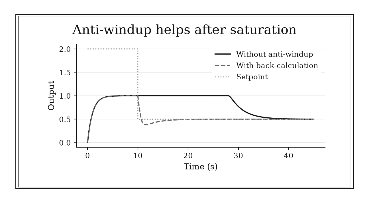
Figure 25.3. The setpoint first demands an unreachable output, then drops to 0.5 at t=10. Back-calculation limits stored integral error and speeds recovery in this constructed PI loop; it cannot make the initial demand reachable.
25.3.4: Always filter derivative action
History
Ideal derivative action solves one problem and creates another: it predicts a fast-moving error before it grows, but its gain rises without limit as frequency increases, so it amplifies sensor noise along with everything else. Alf Isaksson and S. F. Graebe, working at ABB Corporate Research in Västerås, Sweden, made that tradeoff a formal design question in a January 2002 paper titled “Derivative Filter is an Integral Part of PID Design.” They argued a PID controller with realizable derivative action has four design parameters, not three plus an arbitrary default, and showed a poor filter choice could drive excessive control activity.
The equation
A filtered derivative can be written
At low frequency it behaves like (K_d s); at high frequency its gain approaches the finite value
How to read it
is derivative gain and is the filter’s pole, a frequency above which the derivative term’s amplification stops growing. The filtered form behaves like ordinary derivative action at low frequency, but its gain levels off at past , instead of climbing forever like ideal , the way a speedometer needle hits its physical stop instead of spinning off the dial. Placing too low throws away phase lead; too high lets noise and unmodeled dynamics back in.
How to use it
A manufacturing engineer tuning a CNC machine’s position loop has a 1 kHz vibration on the position sensor’s signal, at angular frequency
An ideal differentiator would multiply that vibration’s amplitude by , turning a small sensor wiggle into a large, chattering motor command. The filtered derivative caps that amplification at instead.
Setting several times above crossover, the engineer checks phase contribution against the margin budget, then inspects sensor noise on the bench. Push up toward the vibration’s own frequency to keep the loop feeling responsive, and attenuation relative to the ideal derivative is only at that frequency, about dB, which may leave excessive actuator noise. This is a Specialized rule: it modifies derivative realization to trade phase benefit against finite noise gain.
Chapter Synthesis: Treat Robustness as a Budget
Performance begins with translation. Rise time gives an approximate bandwidth scale, constant disturbance rejection calls for integral action, and dominant-pole reduction requires clear separation plus small modal influence. Each simplification remains provisional until the full response is checked.
Robustness then needs more than one number. Phase margin estimates additional crossover lag, gain margin estimates one multiplicative uncertainty, and peak sensitivity measures the loop’s closest approach to the critical point across frequency. Their usual targets are design screens, not safety certifications.
Implementation spends those reserves. Every delay becomes phase lag at crossover. Digital sampling and zero-order hold add more timing cost. Actuator saturation breaks the linear feedback assumptions and demands anti-windup. Derivative action must be filtered because real sensors contain high-frequency noise.
Across all ten rules, ask:
- What bandwidth and loop structure are actually required by the performance and disturbance specification?
- Which poles, zeros, delays, and uncertainty directions are omitted from the nominal design?
- Do phase margin, gain margin, and peak sensitivity tell a consistent robustness story?
- What changes when the controller is sampled, saturated, quantized, and exposed to sensor noise?
One-Page Control Theory Toolkit
| Recognition cue | Rule to try | What it gives | Role |
|---|---|---|---|
| Rise-time requirement is given | Convert through (t_r_{BW}=O(1)) | Initial bandwidth scale | Independent |
| Constant offset is unacceptable | Add integral action | Low-frequency disturbance rejection | Workflow |
| A low-order model omits poles | Seek at least fivefold decay separation and check residues | Reduction guardrail | Workflow |
| Simple SISO loop needs a phase target | Start near (45)–(60) | Crossover robustness screen | Workflow |
| Plant gain is uncertain | Seek roughly (6) dB gain margin | Factor-of-two screen | Workflow |
| Margins look acceptable but resonance remains | Check (M_s), aiming near or below 2 | Worst-frequency sensitivity | Workflow |
| Latency enters the loop | Subtract (_c) from phase budget | Delay cost | Workflow |
| Continuous controller will be digitized | Sample at 10–20 times bandwidth | Starting update rate | Workflow |
| Integral controller meets actuator limits | Add anti-windup | Saturation recovery | Specialized |
| Derivative or lead uses sensor data | Add a designed derivative pole | Bounded noise gain | Specialized |
Decision Path
- Is the requirement stated in time units? Translate it into a bandwidth interval, then verify the full step response rather than trusting one constant.
- Is the persistent disturbance approximately constant? Add integral structure only if the loop can remain stable and the actuator has enough authority.
- Will a reduced model guide tuning? Compare pole decay, residues, zeros, and full-versus-reduced responses in every important channel.
- Is the loop ordinary SISO with a clear crossover? Use phase and gain margins as starting screens, then inspect peak sensitivity.
- Are there multiple crossovers, unstable poles, or MIMO coupling? Escalate from classical margins to Nyquist, disk, or structured robustness analysis.
- What latency is unavoidable? Convert every component to phase at crossover before raising bandwidth.
- Will the design run digitally? Include sample, hold, computation, jitter, filtering, and quantization in the implemented model.
- Can the actuator saturate or the derivative see noise? Add anti-windup and derivative filtering before nonlinear simulation or hardware tests.
Transfer Problems
1. Turn a transient requirement into a loop budget
A process needs a 10–90% rise time near (0.25) s. Estimate a consistent bandwidth range, choose an initial phase-margin target, and compute the phase cost of (15) ms total delay at the middle of that range. State what full-model effects could invalidate the estimate.
2. Audit classical robustness
A loop crosses 0 dB at phase (-128^). At its (-180^) phase crossing, magnitude is (-7) dB, and computed peak sensitivity is (2.4). Calculate phase and gain margins, convert gain margin to a linear factor, and explain why the sensitivity result still triggers escalation.
3. Prepare a PID design for implementation
A (4) Hz bandwidth PI-D controller updates at (40) Hz, drives an actuator limited to () units, and receives noisy measurements. Evaluate the sampling ratio, propose an anti-windup mechanism and filtered derivative form, and list the nonlinear and timing tests required before deployment.
Where These Ideas Reappear
- Ordinary differential equations: poles, stiffness, timestep stability, and event handling determine whether a simulated loop is numerically trustworthy.
- Signal processing: sample rate, anti-alias filtering, decibels, causal filter delay, and noise normalization are part of every digital controller.
- Optimization: constrained control, reference governors, and model-predictive control turn actuator limits into explicit feasible-set calculations.
- Complex analysis: Nyquist geometry, poles, zeros, and contour ideas connect analytic structure to feedback stability.
- Mechanical and electrical design: bandwidth and damping trade against resonance, sensor dynamics, actuator limits, and unmodeled modes.
- Statistics and uncertainty: robustness margins are only as meaningful as the uncertainty model and confidence attached to plant identification.
Historical Notes and Sources
All ten profiles have verified historical stories. The chapter labels modern coefficient ranges and conventional margin targets separately from the documented historical frameworks.
- Bode and frequency-domain feedback design: digitized record of Bode’s 1945 book; NASA study connecting bandwidth, margins, and performance.
- Minorsky and integral steering control: original 1922 paper; IFAC historical review.
- Evans and root locus: original 1950 paper; U.S. Naval Observatory Library precursor record.
- Nyquist and classical margins: original “Regeneration Theory” paper; NASA loop-shaping and margin analysis.
- NASA and peak-sensitivity retuning: official spacecraft-control report; Bode’s feedback-amplifier book.
- NASA F-8 digital fly-by-wire: contemporary flight-test report; official history, Computers Take Flight.
- Hanus, Kinnaert, and Henrotte on anti-windup: original Automatica paper; ACM bibliographic record.
- Isaksson and Graebe on derivative filtering: original IEE paper; later experimental and analytical study.
- Modern control formulas and design guidance: Åström and Murray, Feedback Systems; feedback loop synthesis notes; University of Michigan Control Tutorials.