Chapter 1 , Algebra: See the Structure Before You Solve
Suppose one quantity rises from 10 to 20 and another rises from 100 to 110. Both have increased by 10. If subtraction is the only lens you use, the changes look identical. They are not. The first quantity doubled; the second rose by only 10 percent.
That contrast reveals algebra’s central habit: identify the structure before beginning the calculation. Algebra is often taught as a sequence of legal operations, expand, collect, divide, substitute, and solve, but experienced problem solvers look first. Is the change additive or multiplicative? Is there a small parameter that makes a local approximation trustworthy? Is a long sum controlled by its endpoints? Is a polynomial’s behavior already visible from its highest power? Will a sign check prevent an invalid transformation?
The seventeen rules in this chapter fall into three families. The first translates change and growth into the right scale. The second compresses calculations by preserving the structure that controls the answer. The third diagnoses algebraic form before a procedure is chosen. Together they support one governing habit: see the structure before you solve.
An exact answer reached through the wrong model, an unstable form, or an invalid sign operation is not rescued by the amount of algebra performed afterward. A short structural check can determine whether the next ten minutes of calculation will be useful.
1.1: Change, Growth, and Local Approximation
Algebra is most useful before the long calculation begins. The five rules in this section show how to choose the right scale for change, translate growth into time, and replace a difficult expression with a controlled local model.
1.1.1: Compare proportional change with ratios, not differences
History
Book V of Euclid’s Elements never once measures a change by subtracting one magnitude from another. Around 300 BCE in Alexandria, Euclid built an entire theory of proportion on the ordering and equality of ratios, letting him compare magnitudes without assigning them modern numerical coordinates at all. That habit survives in a plain modern complaint: two quantities can move by the same raw amount and still not have moved by comparable amounts.
Euclid did not write a percentage-change formula, and he never called ratio a diagnostic tool; the equation below is a modern operational restatement of his organizing idea. What his propositions bought later readers was a question to ask before any subtraction begins: compared to what.
The equation
For an old value and a new value ,
The two measurements are connected:
The scale factor says how many times as large as the old quantity the new one is. Relative change says how much of the old quantity was added or lost.
How to read it
A scale factor of means the new value is one and a quarter times the old one; the matching relative change, , says a quarter of the old value was added. A number below signals shrinkage: means the new value is eighty percent of the old, a twenty percent drop.
Ratios strip away the unit, so the comparison survives a switch from dollars to cents or feet to meters, while a raw difference does not: five dollars more can be a rounding error or a windfall depending on what it is five more than. Near a zero baseline the fraction turns unstable or undefined, and even a well-behaved ratio never speaks to whether the change actually matters, only to its scale.
How to use it
A shopper tracking a weekend price update sees the same five-dollar increase on two items: a kitchen scale moves from to , and a stand mixer moves from to . Subtraction says both got five dollars more expensive and stops there. Ratios separate them:
The scale’s price rose a quarter over its old value; the mixer’s rose one twentieth. If a five percent monthly hike is the store’s normal drift but a twenty five percent hike signals something unusual, the shopper buys the scale today and can afford to wait on the mixer. The catch is the baseline itself: this comparison only works because both items had a nonzero starting price on the tag. An item marked down to nearly nothing beforehand would make the ratio swing wildly for a change of a few cents, exaggerating a trivial move. This is an Independent rule: once a meaningful nonzero baseline is available, it can answer the comparison directly across many applications.
1.1.2: Estimate doubling time from the exponential rate
History
A merchant needed to know, quickly, whether money would double within a working lifetime, not after grinding through a compound-interest table by hand. In 1494, Luca Pacioli’s Summa de arithmetica, printed in Venice, gathered exactly that kind of commercial arithmetic: compound-growth problems used by Renaissance merchants, including a shortcut traditionally associated with estimating doubling time. Speed was the point; a merchant needed a practical horizon, not an abstract rate sitting in a table.
The historical record secures the commercial context and the printed work; it would be anachronistic, though, to hand Pacioli the modern label “Rule of 70” or “Rule of 72.” Pacioli’s text supplies the commercial habit; the mnemonic names, and the derivation below, belong to arithmetic teaching that came after him.
The equation
For continuous exponential growth,
Doubling means , so
If the continuous rate is quoted as per period, then and
For discrete periodic growth,
When is modest, or the highly divisible mental numerator gives a quick estimate of this discrete doubling time.
How to read it
The rate must be written as a fraction of the whole, so a growth rate becomes before it goes anywhere near the formula. Dividing (essentially ) by that fraction turns “growth per year” into “years per doubling.” The relationship runs backward: double the growth rate and the doubling time is roughly cut in half, the way a savings balance growing twice as fast needs half as many birthdays to double. Swap in the whole-number percentage instead of the fraction and the same shortcut becomes periods, easy to do without a calculator.
Whether the growth rate itself stays steady is not something this shortcut checks: it assumes one constant rate held the whole way, and it is silent on a rate that speeds up, slows down, or compounds only once a year rather than continuously.
How to use it
A bakery owner watching revenue grow at a steady a year wants to know whether sales will double before her fifteen-year lease runs out. The mental shortcut gives
just inside the lease. The continuous model checks that estimate:
so the shortcut is off by only about year, comfortably inside the fifteen-year window. If growth instead compounds once a year rather than continuously, the exact discrete figure is
and the alternate mental version, , brackets it just as closely. On the strength of either estimate, the owner plans to renew the lease rather than search for a bigger space now. The one thing the shortcut cannot see is a bad year: if growth stalls or reverses for even one season, the doubling clock resets from wherever revenue actually sits, and averaging a good year against a bad one is not the same as compounding through the sequence she actually lived. This is an Independent rule: under a steady-growth assumption, it directly turns a rate into a useful horizon.
1.1.3: Linearize a small binomial perturbation
History
Multiply five small errors together by hand and intuition usually fails: a chain of overages does not obviously compound to , or to anything a quick guess would land on. In the 1660s in Cambridge, Isaac Newton extended the binomial expansion beyond positive integer powers to fractional and negative exponents, turning a finite algebraic identity into a much broader infinite series and tying algebraic expressions to local approximation.
Newton built the series; the modern instruction to stop after its linear term because a perturbation is small is a later asymptotic reading, expressed in today’s notation and error language. What his expansion bought later users is a way to take just its first two terms and trust the trade: a fast estimate, plus a visible next term that says how much was left on the table.
The equation
For a small, dimensionless ,
Here means that the remaining terms have cubic or smaller scale as approaches zero, with held fixed.
Dropping the quadratic and higher terms gives
The first omitted contribution,
is the quickest warning about the size and direction of the leading correction.
How to read it
Read as a baseline of one multiplied by a small fractional bump every time a stage repeats, like a gear stage that speeds up its output by a hair with each mesh. Raising that repeated bump to the power multiplies the first-order disturbance by : a speed-up at one gear stage becomes roughly a speed-up once the same bump compounds through five stages in a row (). “Small” is not a formality; it means the terms being thrown away are small next to the precision the job actually needs.
Whether that discarded piece is safe to ignore is not something the shortcut checks for you: only comparing with the accuracy the job needs will tell you that.
How to use it
A machinist is checking a five-stage gear train in which each stage speeds up the output shaft by over its input, and needs to know the overall speed-up before running the machine at full load. With and ,
a projected speed-up through the finished train. Before signing off, the machinist checks the first ignored term:
so a sharper estimate is , close to the exact value . Since the downstream equipment’s tolerance on final output speed is , a projected speed-up is well outside it, and the train gets flagged for a stage regrind before the machine runs a full shift rather than after hours of overspeed operation. The rule only holds because the speed-up was small and the same at every stage; a stage that slips differently from the others, or a single mesh far outside , would make the linear estimate misleading exactly when the train’s overall speed matters most. This is an Independent rule: once its small-perturbation condition is checked, it produces a direct estimate in many unrelated settings.
1.1.4: Replace a small exponential by one plus its exponent
History
Because Leonhard Euler folded exponentials into the same organized system as series and logarithms, what once needed a printed table can now be read off one line. His 1748 Introductio in analysin infinitorum, associated with Lausanne and Berlin, gathered functions, infinite series, logarithms, exponentials, and algebraic decompositions into a single computational language and explicitly worked out the power-series expansions behind them.
Euler used those expansions directly, but he wrote before modern convergence tests and floating-point error language existed, so calling this exact instruction, replace a small exponential by one plus its exponent, his own slogan would overstate the case. It is a modern first-pass reading of a series he built for broader purposes. What his systematizing bought later readers is this: near zero, the whole curve of the exponential collapses to a straight line cheap enough to compute by hand.
The equation
The exponential series is
When is small and dimensionless,
The first correction is , which is positive whether is positive or negative.
How to read it
At zero, the exponential function equals and has slope , so near zero its graph tracks the straight line closely, the way a gently curving road looks almost straight for the first few steps onto it. A small positive pushes the true curve a little above that line; a small negative does too, because the next correction, , is always positive whichever way points.
This is a local reading, not a new definition of the exponential: it only holds near zero, and it stops working once grows large, where the line and the curve pull apart fast.
How to use it
A nurse tracking a medication that clears the bloodstream at a steady per hour wants a fast read on how much remains after one hour, before consulting the full decay chart. With ,
so roughly of the dose remains. The correction term,
sharpens that to , close to the true value of about . Both the direction (a small loss) and the scale (about two percent) check out, so the nurse can trust the bedside estimate for a routine one-hour reading. The estimate only holds because the hourly clearance rate is small and steady; over many compounded hours, or with a rate that is not genuinely constant, the gap between the straight-line estimate and the true exponential curve widens, and for a large enough negative the linear formula can even predict a negative concentration, which no real drug level can be. This is an Independent rule: when its small-input condition holds, it directly replaces a difficult exponential across many applications rather than serving only one fixed calculation.
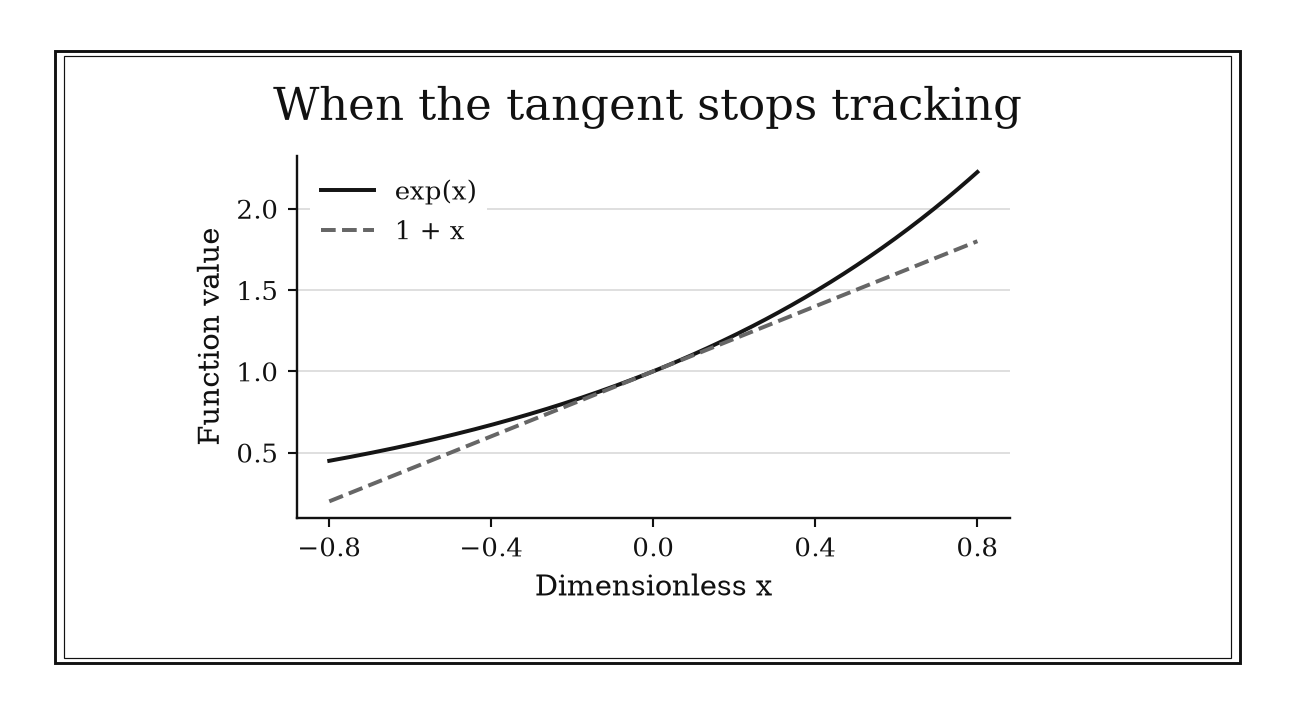
Figure 1.1. For dimensionless x, the exact exponential lies above 1+x on both sides of zero. The gap grows away from zero; judge it against the required tolerance.
1.1.5: Replace log one plus x by x for small x
History
Is this Euler’s rule, or only Euler’s algebra read by later eyes? His 1748 Introductio in analysin infinitorum explicitly develops the series methods this rule depends on, working out the logarithm’s expansion term by term.
Euler wrote before today’s convergence tests and numerical-error vocabulary existed, so treating the compact modern instruction, replace by when is small, as his own phrasing would claim more than the record supports. The structure is his; the slogan is not. What that structure bought later readers is a logarithm collapsed to a single term whenever the input sits close enough to one to trust the shortcut.
The equation
For ,
where is the natural logarithm. At first order,
The leading correction is negative:
How to read it
Think of as a multiplicative factor sitting just above one, the kind of small step a reservoir’s inflow takes when it rises a few percent in a week. The logarithm turns that multiplicative step into an additive one close to the same size: a rise in inflow corresponds to a log change near . Unlike the exponential’s companion rule, this correction subtracts rather than adds, so the plain estimate always runs a touch high for a positive .
How many of these small steps can be chained before the errors pile up is left unanswered here: repeat the approximation across many weeks and the individually tiny quadratic corrections accumulate into something no longer safe to ignore.
How to use it
A hydrologist watching a reservoir’s weekly inflow rise by a steady wants the additive change on a log scale, to add it directly to other small weekly effects tracked in the same report. At first order,
Including the correction term gives
close to the true value . For a single week’s entry in the log, the first-order number is good enough to write down. The hydrologist reaches for the corrected figure only when several weeks of readings are being summed together, because using the plain for every one of many weeks would let the small overestimates from each week quietly compound into a report that overstates total inflow. This approximation converts multiplicative growth into an additive one that is easy to add up, but only as long as stays small; a week with an inflow spike far above needs the exact logarithm, not this shortcut. This is an Independent rule: with a small dimensionless perturbation, it converts multiplicative change into additive change in many settings.
1.2: Compress the Calculation and Expose Dominant Structure
Some algebraic expressions are difficult only because they are written at the wrong level of detail. A long list may be governed by its endpoints, an infinite tail by its first unseen term, and a complicated polynomial by one dominant power. The rules in this section teach a common move: preserve the structure that controls the answer and postpone everything else.
1.2.1: Average the endpoints of an arithmetic list
History
Adding a long list of evenly spaced numbers one term at a time is slow, and slow arithmetic invites mistakes exactly where a business cannot afford one. In the mathematical portion of the Aryabhatiya, composed in 499 CE at Kusumapura in India, Aryabhata gave a procedure for summing arithmetic progressions directly from the number of terms and the two endpoints, without adding each one in turn. The surviving text presents this in compact verse meant to carry a calculation, not in modern symbolic notation.
That supports the connection to evenly spaced lists and their sums; the endpoint-average formula below is a modern algebraic unpacking of his verse, not a quotation from it. What his procedure bought its user was a whole list collapsed into three numbers.
The equation
For an arithmetic progression
with terms and final term ,
In words: sum = number of terms × average of the endpoints.
How to read it
The formula says no term needs handling on its own: pair the first term with the last, the second with the next-to-last, and keep working inward, the way a worker might load a truck from both ends of a numbered rack toward the middle. Constant spacing guarantees every pair adds to the same total, first plus last; an odd count just leaves one middle term sitting at that same average, so nothing special has to be done for it.
The common difference itself never appears in the final formula: it only certifies that the pairing trick is valid. A broken list is invisible to the formula as written: skip an entry, or let the spacing wobble even once, and the pairing argument collapses even though the arithmetic still runs.
How to use it
A lumberyard worker is filling an order for planks cut to linearly increasing lengths, where plank measures board-feet, and the order runs from plank through plank inclusive; the worker needs the total board-feet without walking the rack and adding forty-six numbers by hand. Counting inclusively first,
then averaging the endpoints and multiplying,
gives the total directly. A rough check agrees: about fifty planks averaging about sixty should total somewhere near three thousand, so looks right and goes straight onto the shipping ticket. The one place this shortcut can quietly fail is the count itself: forgetting that both endpoints are included would understate by one, and a gap somewhere in the numbering, say a missing plank , would break the even spacing the whole pairing argument depends on even though the formula would still return a confident number. The worker walks the rack once more for gaps first, then logs the total.
This is an Independent rule: once the list is known to be arithmetic, it produces the desired sum directly rather than serving only as a step in a larger algorithm.
1.2.2: Estimate a geometric tail from its first omitted term
History
A parabolic segment, sliced again and again into ever-smaller triangles, is the artifact at the center of this rule. Around 250 BCE in Syracuse, Archimedes built exactly that construction in Quadrature of the Parabola: an initial triangle, then families of smaller triangles whose combined area shrank by a factor of one quarter at each stage, and he proved the whole infinite pile totals four thirds the area of the first triangle alone.
Archimedes never wrote a modern remainder formula. What his construction establishes is the underlying self-similar geometry: after any stopping point, the pieces still missing repeat the same shrinking pattern seen so far. Reading that leftover from its first missing piece is the modern rule-of-thumb reading of his geometry.
The equation
For a geometric series with , the tail beginning at index is
If the first omitted term is , this becomes simply
How to read it
The first term left out of a sum sets the scale of everything still missing; the factor accounts for the whole shrinking tail that follows it, the way a single quarter-sized copy of a shrinking pile of scraps stands in for every scrap after it. When is small, the leftover tail is barely bigger than that first missing piece. When sits close to , the tail balloons because many later terms still matter almost as much as the first one. For a negative , the tail alternates sign, so its true size can be smaller than a bound built only from magnitudes would suggest.
The formula only measures a leftover that is genuinely geometric: it cannot bound a remainder whose ratio drifts from term to term.
How to use it
A quality-control engineer models a cumulative calibration error as a sum of contributions, each one third of the previous contribution. After recording the initial contribution and four further contributions, the engineer has kept the terms through in
The first contribution not recorded is , worth of the initial contribution, so the uncounted tail is
That number is the total uncounted error, expressed as a fraction of the initial contribution. If the specification requires truncation error below of that contribution, stopping at misses it, since remains uncounted. The engineer records one more contribution before signing off. The calculation assumes that the ratio stays exactly one third; if later contributions follow a different pattern, the geometric tail no longer gives the exact remainder and needs a new bound.
This is an Independent rule: under its convergence condition, it returns the entire remaining error in one calculation.
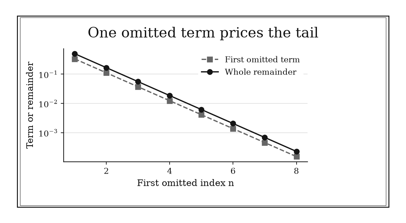
Figure 1.2. For a=1 and r=1/3, the remainder starting at n is 1.5 times the first omitted term. At n=5 the remainder is 1/162. The logarithmic axis shows the constant ratio.
1.2.3: Let the leading term predict polynomial end behavior
History
Getting a large-scale prediction wrong by trusting a small piece of a formula can be expensive long before anyone finishes the exact calculation. Leonhard Euler routinely ordered expressions by their powers rather than treating every term as equally important, a habit running through his 1748 Introductio in analysin infinitorum.
Euler worked with power series and algebraic structure directly, but he wrote before today’s formal limit notation and convergence language, so it would overreach to claim he stated this classroom rule in its present form. What his power-ordering habit bought later readers is a shortcut: far from the origin, a polynomial can be read off its single highest power instead of its full expression.
The equation
If
then
Equivalently, for sufficiently large ,
How to read it
Divide every term of the polynomial by its leading term, . That term becomes exactly , and every lower-degree term shrinks toward zero because it carries a negative power of , the way a small side street stops mattering once you are far enough down the highway. The polynomial’s degree tells you whether the two far ends point the same way or opposite ways; the sign of the leading coefficient tells you which way.
Exactly where “sufficiently large” begins is left unstated. It can sit surprisingly close to the origin or surprisingly far from it, depending on the size of the lower coefficients, and the rule itself gives no warning of the crossover.
How to use it
Before quoting a client, a logistics analyst checks a shipping surcharge model, , where is order weight in some convenient unit, wanting to know whether a very large order’s surcharge will run positive or negative. The leading term, , is odd degree with a negative coefficient, so the model predicts a surcharge falling further negative as order weight grows without bound. At ,
so the leading term already carries the right sign and roughly the right size, and the analyst trusts the formula’s direction for a genuinely large order. The catch shows up at moderate weight:
even though the leading term alone is , because the term still dominates there. Quoting a midsize order using only the leading term would give a client a wildly wrong number and the wrong sign, so the analyst runs the full polynomial for anything short of a genuinely large weight and reserves the shortcut for extremes.
This is an Independent rule: it directly answers the end-behavior question without requiring the rest of a polynomial-solving procedure.
1.2.4: Rationalize a difference of nearby square roots
History
The conjugate trick for two nearby square roots is the artifact at the center of this rule: multiply through by it, and the cancellation trap that ruins a direct subtraction disappears. No dated page records who first reached for it that way. This rule has an evidence gap. Conjugate rationalization is old algebra, and the underlying identity is easy to find in general histories, but the research turned up no dated primary calculation, contemporary teaching text, or documented failure in which a historical actor used this exact nearby-root maneuver to stop digits from cancelling.
A broad history of radicals can show the component identity existed; it cannot show anyone used it this way, for this reason, on a given day. Closing the gap would need a located primary text, in an identifiable hand, applying the conjugate specifically to rescue a near-cancelling subtraction. Until then, the fair description is folk mathematics: a stabilizing trick that spread through calculation practice without a paper trail.
The equation
When both roots exist and their sum is nonzero, multiplying by the conjugate gives the exact identity
When and , read “the magnitude of is much smaller than ”, the denominator is close to , so
How to read it
Subtracting two nearly equal square roots by hand throws away most of the meaningful digits before you even get an answer, the way rounding two almost-identical bills to the nearest dollar can erase the one cent that actually mattered. Multiplying by the conjugate moves the small quantity up into the numerator and divides it by a well-behaved sum instead. This step is exact, not approximate: it is simply the difference-of-squares identity
Only the last step, replacing the denominator by , is an approximation, and it needs to be small next to .
A genuinely large gap between the two roots is not something the rationalized form fixes on its own. The identity stays exact, but the final shortcut denominator becomes the wrong one to trust.
How to use it
A land surveyor checking whether a foundation verified to be square matches its deed measures the plot’s corner coordinates and computes an area of square units where the deed specifies exactly . The side length that would produce the deeded area is , so the correction owed on the measured side is . Rather than rounding and subtracting by hand, which throws away the very digits that matter, the surveyor rationalizes:
The exact rationalized value is about , so the shortcut recovers the scale and several digits immediately, and the surveyor logs the side length as roughly half a hundredth of a unit above the deeded length, well inside the crew’s tolerance. If the discrepancy had instead been large, say a plot closer to than , replacing the denominator by a rounded would no longer track the true value closely, and the exact quotient, not the shortcut, would be the number to trust.
This is an Independent rule: for this recognizable form it directly supplies an exact stable representation, and often the desired estimate, even though the historical evidence for a specific originating episode remains open.
1.2.5: Use logarithms to tame products and powers
History
Trying to directly compare two enormous whole-number totals by multiplying them out by hand invites exactly the kind of arithmetic slip that changes which number is actually bigger. In 1614, John Napier published Mirifici Logarithmorum Canonis Descriptio in Edinburgh. Its tables and rules let astronomers and other human computers replace laborious multiplications, divisions, and root extractions with easier additive operations, a purpose the historical record documents directly.
Napier’s own construction and notation were not identical to a modern algebra textbook’s, so the equations below should not be read as his verbatim phrasing. His tables did the transforming; the notation below only records it: move a multiplicative problem onto an additive scale, do the easier work there, and translate back only if the original units are needed.
The equation
For positive real factors,
and for ,
Because the natural logarithm, and every real logarithm with base greater than , is strictly increasing, exactly when .
How to read it
Logarithms change the grammar of a calculation: products become sums, quotients become differences, and exponents turn into ordinary multipliers out front, the way turning a stack of population figures into their logarithms turns a wall of huge numbers into a short column easy to compare by eye. Because the logarithm is strictly increasing, comparing two logged values is exactly the same as comparing the original quantities, so the originals never need to be written out in full.
Comparing two things safely once either one is zero or negative is outside what logarithms can do; the real logarithm simply has nothing to say there.
How to use it
A public health officer is comparing two rough outbreak projections to decide which needs emergency resources first: one model has cases tripling across generations, the other doubling across generations, and nobody wants to multiply either number out by hand under deadline pressure. Taking natural logs instead,
and since , the doubling model actually produces the larger case count, , despite tripling sounding more alarming generation for generation. The log gap, about , converts back to a ratio of , so the officer reports the doubling scenario as roughly a quarter larger and prioritizes resources there first. The comparison only holds because both case counts are positive; if a model instead tracked a net change that could go negative, taking a real logarithm of it would be invalid, and rounding on the log scale can itself become significant once the huge number is reconstructed, so the officer keeps a few extra digits of precision rather than rounding early.
This is a Workflow rule: it is highly transferable, but the logarithm usually creates an intermediate representation for a later comparison, equation solve, optimization, asymptotic analysis, or numerical evaluation.
1.3: Diagnose Structure Before Choosing a Procedure
The fastest algebra often happens before the formal solution begins. A small change of form can expose the roots, geometry, admissible methods, or hidden hazards of a problem. The seven rules in this section are therefore less about executing an algorithm than about deciding what kind of problem is actually in front of you.
1.3.1: Make a quadratic monic before reading its structure
History
A quadratic scaled up by an arbitrary leading coefficient hides its own root pattern until that scale is stripped away. Dividing it through by that coefficient turns two of the remaining coefficients directly into the sum and the product of its roots. Around 820 in Baghdad, al-Khwarizmi classified quadratic equations into verbal types and solved them by operations he called restoration and balancing; for a type equivalent to , his geometric demonstration added pieces to complete a square and made the unknown readable as a length. He never wrote , nor did he state dividing by the leading coefficient first; that connection is a modern reconstruction that exposes why a unit-scale squared term makes a quadratic’s structure visible.
The equation
For , divide every term by :
[ ax^2+bx+c=0 x^2+ba x+ca=0. ]
If the roots are and , the monic form immediately gives
[ r_1+r_2=-ba, r_1r_2=ca. ]
“Monic” simply means that the coefficient of the highest power is .
How to read it
Normalizing separates two kinds of information: the original sets an overall vertical scale, while the ratios and control the root relationships. Once is divided away, the coefficient of is the negative root sum and the constant is the root product, so sign and size patterns become visible at a glance.
Not every feature of the original function survives this division: rescaling by changes its vertical scale and flips it upside down when is negative, even though the zeros themselves stay exactly where they were.
How to use it
A homeowner has a contractor’s equation for a garden path’s edge positions, , and wants the two edge locations without hunting for a formula. Dividing every term by ,
[ x^2-5x+6=0, ]
the roots must sum to and multiply to . The pair and fits, so
[ x^2-5x+6=(x-2)(x-3), ]
and the path’s edges sit at and . The homeowner marks the stakes without computing a discriminant. The move is exact, but if the leading coefficient is itself a rough field measurement rather than a clean , dividing by it can magnify whatever error was already there, so the crew checks the original measurement first and only then trusts the divided-through equation.
This is a Workflow rule: it rarely finishes the calculation, but it improves several procedures that may follow.
1.3.2: Complete the square to read a quadratic’s geometry
History
Was al-Khwarizmi solving an equation, or building a shape? In the same Baghdad treatise, around 820, for equations equivalent to , he arranged rectangular pieces around a square and supplied the missing corner pieces so the whole figure became a larger, completed square, letting the unknown be read off as a length. His documented act stops at the completed square. Coordinate geometry did the rest, turning that same figure into a graph’s minimum, maximum, or vertex with notation he never had.
The equation
For ,
[ ax^2+bx+c =a(x+)^2 +c-. ]
Equivalently, in vertex form,
[ ax2+bx+c=a(x-h)2+k, h=-, k=c-. ]
The point is the parabola’s vertex.
How to read it
Vertex form turns three coefficients into three geometric facts: marks the axis of symmetry, is the extreme value reached there, and the sign of says which way the parabola opens and whether is a minimum or a maximum. Move an equal distance either way from and the squared term returns the same value both times.
The form also previews real zeros: for , rules them out, gives one repeated zero, and allows two. Whether the vertex answers the actual question is separate from finding it: on a restricted domain, the true extreme value can sit at a boundary instead.
How to use it
A track coach has modeled a sprinter’s split-time variance across repeated intervals as , where counts the interval number, and wants the least variance the model predicts before scheduling a taper. Factoring from the first two terms, then completing the square:
[]
Since , the modeled variance never drops below , reached at interval , so the taper is scheduled there without plotting another point. The vertex only answers the question if interval falls inside the session actually run: a workout that stops at interval has its true minimum at whatever endpoint it stopped at, not at the untested .
This is a Workflow rule: the transformation is widely reusable, but its purpose is to enable a later geometric, optimization, sign, or root judgment.
1.3.3: Factor before reaching for the quadratic formula
History
Two techniques for solving the same equation can each have a long documented past without proving which one a solver reached for first. This rule has an evidence gap. Factoring and general quadratic-solving methods both have deep histories, but the research found no dated primary calculation, contemporary teaching text, or documented failure pinning “try factoring first” down as a lesson some historical figure actually taught. A broad history showing both techniques existed side by side does not prove any solver used this exact method-selection habit. Attaching the advice to a famous algebraist for color would turn a plausible guess into an invented story; the honest position is that it is a modern workflow convention whose mathematics is sound even though its origin story is not yet documented.
The equation
Factoring rewrites a sum as a product. Two common patterns are
[ ab+ac=a(b+c) ]
and
[ x^2-(r+s)x+rs=(x-r)(x-s). ]
Once an equation has the form
[ U(x)V(x)=0, ]
the zero-product property says that or .
How to read it
A factor sitting in plain sight is compressed information about where the solutions are, the way spotting a shared tool already out on the workbench beats digging through the whole toolbox. A common factor exposes one whole branch of answers, a difference of squares exposes a symmetric pair, and a pair of integers matching the coefficients’ sum and product can hand over both roots at once. “Factor first” does not mean guess forever. Run one quick scan for a greatest common factor, a difference of squares, or an obvious integer pair, then move on.
A failed scan proves nothing about existence: plenty of quadratics with perfectly good real or complex roots simply do not factor over the integers.
How to use it
A tutoring center coordinator is walking a student through and wants the fastest path to the answer rather than the quadratic formula by default. Both terms share the factor , so
[ 3x(2x-5)=0, ]
giving or . The quadratic formula reaches the same answers, but only after a discriminant and a fraction are simplified along the way. The coordinator warns against dividing the equation by to simplify it, since that silently erases the solution ; keeping the equation at zero and using the zero-product property protects both roots. When a quick scan turns up nothing, the student moves straight to the discriminant instead of hunting for a factor that may not exist.
This is a Workflow rule because it selects a cheaper route when one is available; it is not an independent solution method for every quadratic.
1.3.4: Use the discriminant to triage quadratic roots
History
Solving an equation all the way through only to discover the answer was never real is wasted work that a smaller check could have caught first. In 1545, Girolamo Cardano’s Ars Magna confronted the different algebraic cases that appear as coefficients change, presenting systematic solutions of cubic and quartic equations, some passing through quantities now interpreted as negative and complex numbers. Cardano never used a symbol , nor did he lay out today’s three-line quadratic triage. His documented contribution is the sustained encounter with changing root cases; folding that same case distinction for a quadratic into the sign of one coefficient expression is a modern shorthand for his struggle, not his own notation.
The equation
For
[ ax^2+bx+c=0, a, ]
the discriminant is
[ D=b^2-4ac. ]
For real coefficients,
[]
It is the quantity beneath the square root in .
How to read it
The discriminant is a classifier before it is anything else: its sign says whether a parabola crosses the horizontal axis twice, just grazes it once, or never reaches it. With rational coefficients, a positive perfect-square discriminant points to rational roots, a positive non-square to irrational ones.
Values near zero deserve caution: they mark the boundary between two roots and none, so a small coefficient change nearby can flip the classification.
How to use it
A bridge inspector has a quadratic model, , for where a stress curve might cross zero along a beam, and wants to know whether to expect a crossing before running a full numeric solve. Computing the discriminant,
[ D=2^2-4(3)(5)=4-60=-56, ]
the negative result says immediately that the stress curve never actually reaches zero anywhere along the beam, so the inspector stops there rather than launching a root search. Because the coefficients came from rounded field measurements, the inspector also checks how close sits to zero relative to that measurement uncertainty; is safely negative even after reasonable rounding, but a value near zero means the classification waits on tighter data first.
This is a Workflow rule: it is a self-contained diagnosis, yet its chief role is to select the next procedure, or show that no further procedure is needed for the question asked.
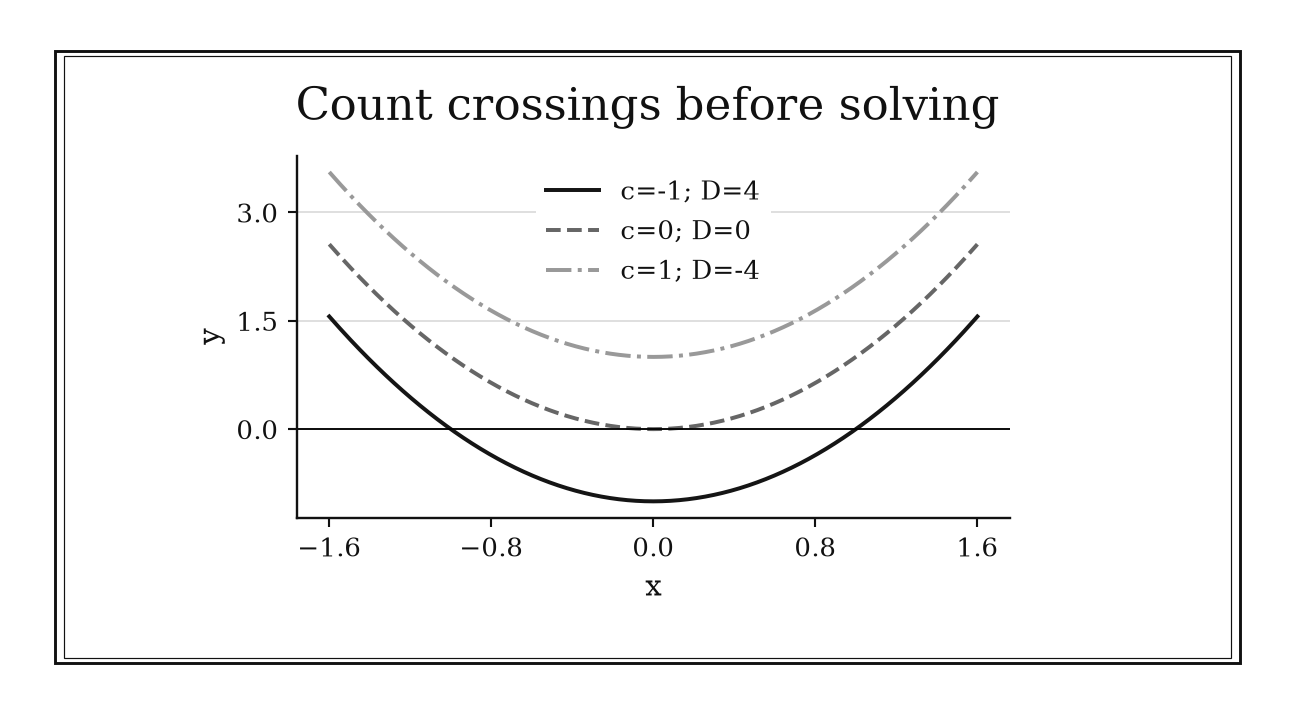
Figure 1.3. The constructed family y=x²+c has two, one repeated, or no real roots as c is negative, zero, or positive. Near discriminant zero, small coefficient changes can alter the classification.
1.3.5: Use the rational-root theorem as a shortlist
History
Searching every possible rational root of a polynomial by trial is hopeless; the candidates are infinite until something narrows the field. Carl Friedrich Gauss’s Disquisitiones Arithmeticae, tied to Leipzig in 1801, systematized congruences, divisibility, and the arithmetic of polynomial forms, and its structural treatment of integer factors made finite divisibility tests a natural first screen before more general algebraic methods. Gauss never stated the present classroom advice in these words; his documented contribution is the structural treatment of divisibility itself. The rule-of-thumb connection modernizes that structure for a narrower job: shrinking infinitely many possible rational roots to a short, testable list.
The equation
For an integer-coefficient polynomial
[ P(x)=a_nx^n++a_1x+a_0, ]
if a rational root is written in lowest terms as , then
[ pa_0, qa_n. ]
If , first factor out the largest power of , record zero as a root, and apply the theorem to the remaining polynomial. Otherwise, every rational root must appear among
[ , ]
after duplicate fractions are reduced.
How to read it
The theorem hands over a necessary condition, not a promise, the way a short list of known combinations narrows a stuck padlock without opening it: a candidate missing from the list cannot be a rational root, but one on the list is only eligible and still needs testing by substitution or synthetic division. The constant term controls possible numerators, since it is what remains at ; the leading coefficient controls possible denominators, since clearing powers of forces divisibility at the other end.
A short list is not guaranteed: when both outer coefficients carry many divisors, the candidate list can grow too long to be practical.
How to use it
A tank designer has a cubic volume-balance equation, , for a design parameter , and needs exact balance points rather than a numerical guess. Possible reduced rational roots, from factors of over factors of , are
[ , , , , , , , . ]
Testing gives , exposing as a factor; synthetic division gives
[ 2x3-3x2-8x+12=(x-2)(2x-3)(x+2), ]
so the balance points are , , and . Only the positive values matter physically, so the designer chooses between and using the design’s other constraint. The theorem only screens rational candidates: had none of the sixteen candidates worked, that would rule out a rational answer but say nothing about a real or complex one, leaving a numerical solver as the next step rather than a conclusion that no design exists.
This is a Workflow rule: it narrows a search and verifies promising exact factors, but it does not finish the problem until the candidates are tested.
1.3.6: Let denominator factors dictate partial fractions
History
Get the setup for a rational function’s decomposition wrong, and every integral, transform, or system solution built on it inherits the mistake. Leonhard Euler’s 1748 Introductio in analysin infinitorum treats rational functions directly through the factors of their own denominators, unlike the series expansions used elsewhere in this chapter: this is direct historical use of the governing structure, not a later reading layered onto work built for something else. Today’s concise template packages that same practice; what it buys is a decomposition whose shape is dictated before a single coefficient is computed.
The equation
For a proper rational function with distinct linear factors,
[ =+. ]
A repeated factor requires every power,
[ + ++, ]
while an irreducible quadratic factor requires a linear numerator for each .
How to read it
Each factor in a denominator earns its own family of terms above the line, the way sorting mail into boxes gives each address its own simpler pile instead of one tangled bag: how many times a factor repeats decides how many powers must appear, and its degree, the highest power present in that factor, decides the numerator’s degree over each one. An irreducible quadratic factor, one that cannot be split into real linear factors, needs a linear numerator instead of a constant. The unknown coefficients never change this template; they only pick out which member of it equals the function at hand.
What the template will not warn you about is a repeated or irreducible-quadratic factor hiding in the denominator: forcing the same distinct-linear pattern onto either one leaves coefficients with no consistent solution.
How to use it
Reducing a vibration model to the transfer function , a control-systems engineer needs it split before applying a standard inverse-transform table. The denominator’s two distinct linear factors dictate the template:
[ =+. ]
Clearing denominators gives ; gives , and gives , so
[ =-. ]
Each piece is then looked up separately in the transform table. The setup holds only at the domain’s exclusions, ; if a later model revision turns one factor into a repeated one, this same two-term template would misrepresent the system’s response at that pole.
This is a Workflow rule: denominator-driven setup is one step in integration, inverse transforms, recurrence solving, and system analysis, but it transfers across all of those larger calculations.
1.3.7: Cross-multiply inequalities only after checking signs
History
A warning that is mathematically airtight can still have no verified birthday. This rule has a documented evidence gap. Sources on ancient proportion theory document plenty of ratio reasoning, but the research did not locate a primary episode where a consequential mistake was traced specifically to cross-multiplying by an expression of unknown sign. Treating any old ratio calculation as this rule’s origin would confuse the long history of proportion with the narrower history of this particular safety warning. What would close the gap is a dated calculation, a contemporary teaching text, or a recorded failure showing the warning itself at work. Until then, transparency about the missing anecdote is more honest than inventing one.
The equation
For nonzero and , begin with
[ ab<cd. ]
Multiplication by gives two different cases:
[ bd>0 ad<bc, bd<0 ad>bc. ]
The same rule applies to : multiplication by a positive quantity preserves the comparison, while multiplication by a negative quantity reverses it.
How to read it
Cross-multiplying is multiplication by the product of two denominators, so whether it is even legal depends on the domain, and which direction the inequality points afterward depends on that product’s sign. A constant positive denominator is easy; a variable denominator changes sign at its own zeros and splits the number line into intervals worth checking separately.
A denominator equal to zero is never part of the solution. Tracking a denominator that changes sign partway through the domain is exactly what one global cross-multiplication cannot do; only splitting at its zeros can.
How to use it
A bookkeeper is solving a scaling inequality, , for a signed adjustment factor that a ledger entry is divided by, so the entry’s effective multiplier is (positive for a credit correction, negative for a debit one); company policy caps any effective multiplier at , and the bookkeeper needs the full valid range before reconciliation software accepts an entry. The domain excludes . For , multiplying by preserves the sign:
[ 1<2xx>. ]
For , multiplying flips it:
[ 1>2x, ]
true for every negative , so the valid range is
[ x(-,0)(,). ]
Both pieces go into the reconciliation entry, unlike the single positive interval a careless cross-multiplication would give, which would have discarded a whole valid branch of legitimate debit corrections.
This is a Workflow rule, specifically a guardrail. It does not solve rational inequalities by itself, but it prevents an otherwise valid transformation from reversing the answer or admitting an undefined point.
Chapter Synthesis: A Structural First Pass
The rules in this chapter do not form one long algorithm. They form a set of questions to ask before an algorithm is chosen.
Start with scale: decide whether the comparison is additive or multiplicative, and whether a genuinely small dimensionless quantity permits a local model. Then look for compression: symmetry, repeated ratios, dominant terms, and changes of representation can replace long arithmetic with a shorter equivalent question. Finally, diagnose structure before selecting a procedure. Normalization, factor patterns, coefficient tests, denominator structure, and sign partitions reveal what an exact method must preserve.
The deeper habit is to separate four questions:
- What representation exposes the controlling structure?
- Is the proposed step exact, approximate, or merely diagnostic?
- What assumption makes it legal?
- Does it answer the question, or does it prepare the next calculation?
That last distinction prevents two opposite errors. An independent estimate should not be buried under unnecessary computation. A workflow guardrail should not be mistaken for a finished answer.
One-Page Algebra Toolkit
| Recognition cue | Rule to try | What it gives | Role |
|---|---|---|---|
| Equal differences but different baselines | Compare with ratios | Scale factor or relative change | Independent |
| Steady exponential rate | Divide () by the rate | Doubling horizon | Independent |
| Small change inside a power | ((1+x)^a+ax) | First-order power-law response | Independent |
| Small exponent | (e^x+x) | Local growth or attenuation | Independent |
| Factor near one inside a logarithm | ((1+x)x) | Additive form of multiplicative change | Independent |
| Evenly spaced finite list | Average the endpoints | Exact sum | Independent |
| Fixed-ratio convergent tail | First omitted term over (1-r) | Exact remainder or error scale | Independent |
| Large-input polynomial behavior | Keep the leading term | Tail direction and scale | Independent |
| Difference of nearby radicals | Multiply by the conjugate | Exact stable form and local estimate | Independent |
| Huge product or power | Take logarithms | Additive comparison scale | Workflow |
| Quadratic obscured by common scale | Make it monic | Root-sum and root-product structure | Workflow |
| Quadratic geometry or extremum | Complete the square | Vertex, bound, and sign information | Workflow |
| Visible common or integer factor | Factor briefly before general methods | Exact solution branches | Workflow |
| Need root type before root values | Compute (b^2-4ac) | Real/repeated/complex classification | Workflow |
| Integer polynomial may have rational factors | Build the rational-root shortlist | Finite candidate set | Workflow |
| Rational function with factored denominator | Mirror its factors in the template | Partial-fraction setup | Workflow |
| Variable denominators in an inequality | Split by denominator zeros and signs | Valid order-preserving transformation | Workflow guardrail |
Decision Path
- Is the question about change? Use a ratio when the baseline matters. If the model is exponential, translate rate into doubling time.
- Is there a small, dimensionless quantity? Match the surrounding function: binomial power, exponential, logarithm, or nearby radical. Estimate the first omitted correction.
- Is there a long sum or tail? Check for constant spacing or a constant ratio before touching individual terms.
- Is magnitude enormous or multiplicative? Move to a logarithmic representation.
- Is the object a polynomial? Use the leading term for distant behavior. For a quadratic, normalize, inspect for factors, and compute the discriminant before choosing a full root procedure. For a higher-degree integer polynomial, use the rational-root theorem only as a finite screen.
- Is the object rational? Factor the denominator. If decomposing a function, let the factors build the partial-fraction template. If solving an inequality, let the factor zeros build the sign chart.
Transfer Problems
1. Same gain, different meaning
A small organization adds 200 customers, growing from 400 to 600. A large organization adds the same 200, growing from 20,000 to 20,200. Compare the changes on the appropriate scale. Then state why a raw difference answers a different question.
2. Build an approximation budget
Estimate each quantity without first using a calculator:
[ (1.01)^8,e^{-0.04},(1.04). ]
For each estimate, write the leading omitted correction and decide whether a requested accuracy of (10^{-3}) is plausible.
3. Choose the procedure before solving
For each expression, name the first structural rule you would apply and explain why:
[ 4x^2-20x+24=0, , . ]
Do not finish the calculations until you have stated the relevant domain exclusions, factor structure, or root diagnostic.
Where These Ideas Reappear
- Geometry: ratios become similarity and square-cube scaling.
- Calculus: the binomial, exponential, logarithmic, and radical rules become first-order Taylor models with explicit remainders.
- Analysis: geometric tails and leading-term comparisons become convergence and asymptotic tools.
- Complex analysis: negative discriminants and logarithms require attention to complex roots and branches.
- Linear algebra and numerical methods: rationalization anticipates the broader principle of reformulating a calculation to avoid cancellation or poor conditioning.
- Number theory: the rational-root shortlist is powered by divisibility, while finite candidate screens reappear throughout discrete mathematics.
Historical Notes and Sources
Sources for the historical accounts in this chapter follow. The evidence-gap entries support the mathematics of their rules without claiming an unverified origin event.
- Euclid and ratios: Book V of Euclid’s Elements, Clark University edition.
- Pacioli and commercial doubling: Library of Congress copy of the 1494 Summa; Library of Congress guide to early accounting practice.
- Newton and the generalized binomial expansion: The Newton Project; MacTutor, “The Rise of Calculus”.
- Euler’s 1748 Introductio: Euler Archive digital text and record; MAA Mathematical Treasures discussion.
- Aryabhata and arithmetic progressions: MacTutor biography; MacTutor history of Indian mathematics.
- Archimedes and geometric accumulation: The Archimedes Palimpsest project; Harvard translation and study materials.
- Napier and logarithms: Smithsonian Libraries digitization of the 1614 Descriptio; University of Oklahoma Galileo Collection exhibit.
- Al-Khwarizmi and quadratics: MacTutor translation and discussion; MacTutor biography.
- Cardano and changing root cases: MacTutor history of quadratic, cubic, and quartic equations.
- Gauss and divisibility structure: Library of Congress digitization of Disquisitiones Arithmeticae; Smithsonian Libraries digitization.
- Evidence-gap mathematics: OpenStax on radicals and rational exponents, quadratic equations, and linear inequalities. These support the mathematics but do not establish exact historical origin events for the three gap profiles.